User guide

In this page, we will give a detailed explanation of this python package. All the crucial functions in each module will be covered.

Fundamental algorithm

This section introduce the basic algorithm we used for the various speckle tracking techniques. Most functions described in this section comes from the corefun module.

Cross-correlation

In image processing, cross-correlation is a measure of the similarity of two images. For template matching, the template image moves along the surface of the reference image. At each position, a cross-correlation calculation is conducted. The output of these cross-correlation calculations is a coefficient matrix. This matrix is often used to estimate how the two images resemble. According to the mode of cross-correlation used, usually, the largest or smallest value in the coefficient matrix corresponds to the position the template image and the reference image resemble the most.

Animation of the cross-correlation sliding a template over an image. (Image is from wikipedia.)

The normalized cross-correlation is used to obtain the coefficient matrix in this package. This matrix can provide the pixel-wise location of the highest correlation. It is also used to obtain the sub-pixel registration, which we will cover in the next section Sub-pixel registration.

If \(t(x,y)\) is the template image, \(f(x,y)\) is the sub-image of the raw image which is to be cross-correlated, then the normalized cross-correlation is:

\[R(x,y) = \frac{1}{n} \sum\limits_{x',y'}\frac{1}{\sigma_{t}\sigma_{f}} (t(x',y') - \bar t)(f(x+x', y+y') - \bar f(x, y))\]

where \(n\) is the number of pixels in \(t(x', y')\) and \(f(x+x', y+y')\), \(\bar t\) and \(\bar f(x, y)\) are the average of \(t(x', y')\) and \(f(x+x', y+y')\), respectively.

The OpenCv-Python (cv2) package is heavily used in this package. Especially, we use the existing cv2.matchTemplate function to calculate the cross-correlation matrix. The standard normalized cross-correlation shown above corresponds to the TM_CCOEFF_NORMED method for the existing template matching function. Other methods haven’t been implemented in this package.

For more information of the template matching in OpenCv-Python (cv2) package, please refer to this link.

Sub-pixel registration

We provide three sub-pixel registration methods at present. They are the differential approach (the default method), Gaussian peak locating, and parabola curve peak locating. Other methods can be easily implemented if required.

The subpixel registration functions are defined in corefun module.

Default method

The default sub-pixel registration method can be found in [defaultref1] and [defaultref2].

This method can be described in the following. The method can be described in the following. We assume the coefficient matrix obtained from the cross-correlation to be \(R(x,y)\). It has the pixel-wise maximum value at \((x_0, y_0)\). \((x_0, y_0)\) is the index of the pixel. We assume the cross-correlation has its maximum value at the position of \((x_0+\delta x, y_0+\delta y)\). Then we have:

\[ \begin{align}\begin{aligned}\delta x = \left( \frac{\partial^{2} R}{\partial y^{2}} \frac{\partial R}{\partial x} - \frac{\partial^{2} R}{\partial x \partial y} \frac{\partial R}{\partial y} \right) \left( \left( \frac{\partial^{2} R}{\partial x \partial y} \right)^{2} - \frac{\partial^{2} R}{\partial x^{2}} \frac{\partial^{2} R}{\partial y^{2}} \right)^{-1}\\\delta y = \left( \frac{\partial^{2} R}{\partial x^{2}} \frac{\partial R}{\partial y} - \frac{\partial^{2} R}{\partial x \partial y} \frac{\partial R}{\partial x} \right) \left( \left( \frac{\partial^{2} R}{\partial x \partial y} \right)^{2} - \frac{\partial^{2} R}{\partial x^{2}} \frac{\partial^{2} R}{\partial y^{2}} \right)^{-1}\end{aligned}\end{align} \]

To discrete the above partial differential operators, the central difference scheme is used.

Gaussian peak finding method

Both this method and Parabola peak finding method can be find in [gaussref1].

Assuming the coefficient matrix \(R(x, y)\) can be fitted by a 2D Gaussian function, the peak location of the fitted function is:

\[ \begin{align}\begin{aligned}x_m = x_0 + \frac{\ln(R(x_{0}-1, y_{0}))-\ln(R(x_{0}+1, y_{0}))}{2\ln(R(x_{0}+1, y_{0}))-4\ln(R(x_{0}, y_{0}))+2\ln(R(x_{0}-1, y_{0}))}\\y_m = x_0 + \frac{\ln(R(x_{0}, y_{0}-1))-\ln(R(x_{0}, y_{0}+1))}{2\ln(R(x_{0}, y_{0}+1))-4\ln(R(x_{0}, y_{0}))+2\ln(R(x_{0}, y_{0}-1))}\end{aligned}\end{align} \]

where \(x_0\) and \(y_0\) are the pixel indices in the two dimensions with the maximum value of \(R(x, y)\).

Parabola peak finding method

Resemble to Gaussian peak finding method, parabola peak finding method assumes the coefficient matrix \(R(x, y)\) can be fitted by a 2D parabolic function. The peak location of the fitted function is:

\[ \begin{align}\begin{aligned}x_m = x_0 + \frac{R(x_{0}-1, y_{0})-R(x_{0}+1, y_{0})}{2R(x_{0}+1, y_{0})-4R(x_{0}, y_{0})+2R(x_{0}-1, y_{0})}\\y_m = x_0 + \frac{R(x_{0}, y_{0}-1)-R(x_{0}, y_{0}+1)}{2R(x_{0}, y_{0}+1)-4R(x_{0}, y_{0})+2R(x_{0}, y_{0}-1)}\end{aligned}\end{align} \]

where \(x_0\) and \(y_0\) are the pixel indices in the two dimensions with the maximum value of \(R(x, y)\).

[defaultref1]

Fisher, G. H., & Welsch, B.T. “FLCT: a fast, efficient method for performing local correlation tracking.” Subsurface and Atmospheric Influences on Solar Activity. Vol. 383. 2008.

[defaultref2]

Qiao, Zhi, et al. “Wavelet-transform-based speckle vector tracking method for X-ray phase imaging.” Optics Express 28.22 (2020): 33053-33067.

[gaussref1]

Debella-Gilo, M, and Kääb, A. “Sub-pixel precision image matching for measuring surface displacements on mass movements using normalized cross-correlation.” Remote Sensing of Environment 115.1 (2011): 130-142.

Image match

The Imagematch() function from the corefun module is the basic function this package calls to do the cross-correlation. It wraps cv2.matchTemplate function and several sub-pixel registration methods. The two mandatory inputs are two images, im1 and im2. im2 by definition must be smaller than im1.

delayX, delayY, res_mat = Imagematch(im1, im2)

This function returns tracked shifts (delayX and delayY) betweeen im1 and im2 and also the related cross-correlatin coefficient matrix res_mat (if res is True).

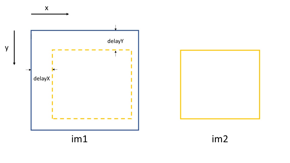
Image normalization

We do normalization to mitigate the impact of the non-uniformity of the images.

Wherever to do the normalization, the basic function to call is NormImage(). The process is as follows.

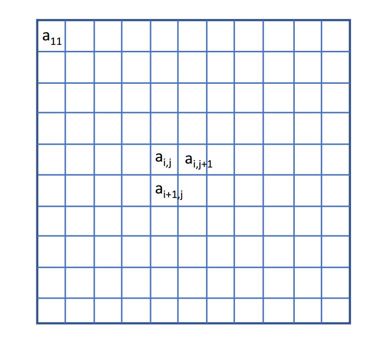
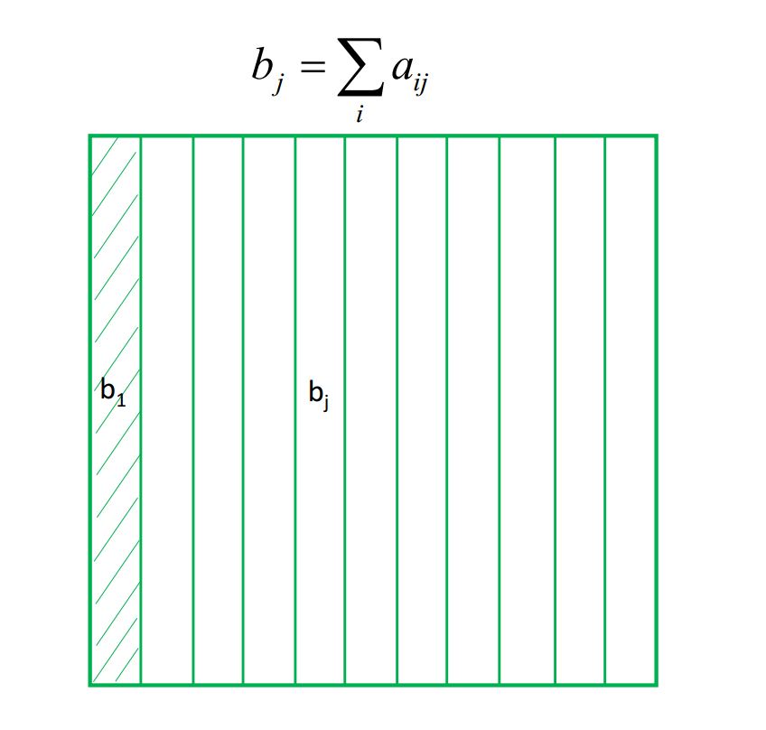
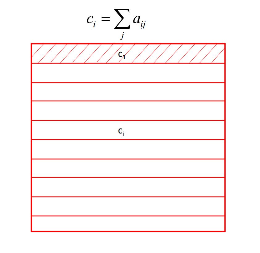
\(b_j\) and \(c_i\) are the partial sums of each column and row of the raw image, respectively.

\(\bar{a}_{i,j}\) is generated as the following. First, for every index \(j\), the column of the raw image, \(a_{i,j}\), divides \(b_j\). Second, after the above first step, for every index \(i\), the row of the generated image divides \(c_i\).

Then we do the common normalization. \(\bar{a}\) is the mean value of \(\bar{a}_{i,j}\), \(\sigma\) is the std of \(\bar{a}_{i,j}\), then we have each element of the final generated image as \((\bar{a}_{i,j}-\bar{a})/\sigma\).

As the images shown in the following, the main purpose of doing normalization is to get rid of the “wrinkles” come from the incident beam. If the normalization is not effect to the raw images, we recommend to do the normalization to the stiched images later. Besides, if the incident beam is clean enough, there is no need to do the normalization.

Auxiliary functions

We provide functions read_one() and crop_one() in the corefun module to help the user read one image into the memory and see it and crop it.

To call read_one() function, you need to input the file path of the image that you want to read. If ShowImage is set to be True, then it will show the loaded single image automatically after you call this function.

The crop_one() function has a parameter ROI to set the region of interest to be cropped from the loaded raw image. To correctely call this function, the user need to use read_one() function to load the raw image into memory. The following is the an example of a piece of codes the user need to crop the raw image and to show it. The raw image is loaded into memory and assigned to im_raw. Then im_raw is paased to read_one() function. The ShowImage parameter is the same as read_one().

im_raw = read_one(filepath=IMAGE / FILE / PATH, ShowImage=True)
ROI = [750, 1500, 500, 2000]    #[y_start, y_end, x_start, x_end]
im_crop = crop_one(im_raw, ROI, ShowImage=True)

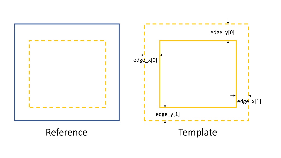
ROI=[y_start, y_end, x_start, x_end]. The first two parameters of ROI is the start and the end position of y coordinate, the last parameters of ROI is the start and the end position of x coordinate. The start and the end coordinates are shown below.

Note

Only .tiff and .png files are considered at present. If it is possible, it is preferred to convert your images in the data set to .tiff files.

The Hartmann_mesh_show() function is used to show the boxes chosen for the Hartmann-like data processing method.

from spexwavepy.corefun import read_one, crop_one, Hartmann_mesh_show

ROI_ref = [540, 1570, 750, 1800]
im_full = read_one(filepath=IMAGE / FILE / PATH, ShowImage=False)
im_crop = crop_one(im_full, ROI_ref, ShowImage=False)

The shape of the cropped image is 1050(x) \(\times\) 1030(y). The centres of the boxes used for Hartmann-like data processing is defined as:

import numpy as np
x_cens = np.arange(50, 1050, 50)
y_cens = np.arange(60, 1000, 50)

The four mandatory inputs for Hartmann_mesh_show() function are the image to be processed, the mesh grid of box’s centre coordinate for x and y axis and half size of the chosen box.

x_cens, y_cens = np.meshgrid(x_cens, y_cens)
size = 15
Hartmann_mesh_show(im_crop, x_cens, y_cens, size)

plt.show()

In the above code, the width and height of the box are 2*size=30 both. After evoking plt.show(), the boxes used for Hartmann-like data processing are shown.

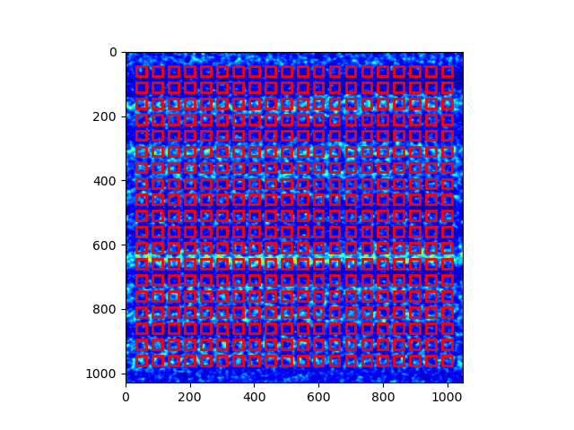
Image stack and its functions

To use this python package to process the experiment data, you need to load the acquired image data into an image stack. A class is defined to achieve this. Other reltated functions are also been covered in this imstackfun module.

Image stack

From all the given examples, the first thing you need to do is to creat the Imagestack class. It is the image stack serves as a container for the acquired images which are read into the memory.

A typical excerpt of the code to create the Imagestack class is as follows:

from spexwavepy.imstackfun import Imagestack

folder_path = "/Your/data/folder/path/"
ROI = [0, 2048, 0, 2048]
imstack = Imagestack(fileFolder=folder_path, ROI=ROI)

Two parameters are needed as the input to create the Imagestack class. fileFolder is the data folder path for the acquired images, ROI is the region of interest to be cropped from the raw image. ROI=[y_start, y_end, x_start, x_end]. Its defination can also be found in the above section.

Data reading

There are other properties that are automatically defined when initiating the Imagestack class. Most of them relate to the raw data reading.

fstart defines the number of the first image to be loaded into memory. The default value is 0. That means the first image. Otherwise, data loading will be start from image number of fstart.

fstep defines the step of the data reading when iterating over the dataset. The default value is 1. That means to read every image until it reaches the designated end.

fnum defines the total number of images to be read in the dataset. The default value is negative. That means to read all the files in the dataset. If it is a positive number, the number of images reading into memory equals the value of fnum.

After properly defining the above attributes, the following code can be used to read the data:

imstack.read_data()

The above code is not mandatory. The raw data can be loaded later as long as the rawdata is None.

The read_data() method of the Imagestack class is called to load the data into the memory. After the invoking of this method, the raw data is stored in the read-only rawdata attribute, the same raw data is also stored in the data attribute. This attribute can be modified when other methods are called.

In general, read_data() method reads from the image start with the number of fstart, with the loading step of fstep, total image number of fnum.

Preprocessing of the images

There are some other methods defined in Imagestack class. They are mainly used to preprocess the raw images in the image stack.

Normalization

The norm() method is called to normalize the raw images in the image stack. The normalization algorithm used for each image is described in the above section.

Note

There are two places in this package to do the normalization. One is to normalize the raw images, the other one is to normalize the stitched images (see in the following sections for the Tracking class). Usually, we only choose one place to do the normalization.

If you want to do the normalization for the raw images in the dataset, set the normalize attribute to True.

imstack.normalize = True

Then when you call the read_data() function, the raw images will be normalized during data loading.

Another way is to explicitly call norm() method:

imstack.norm()

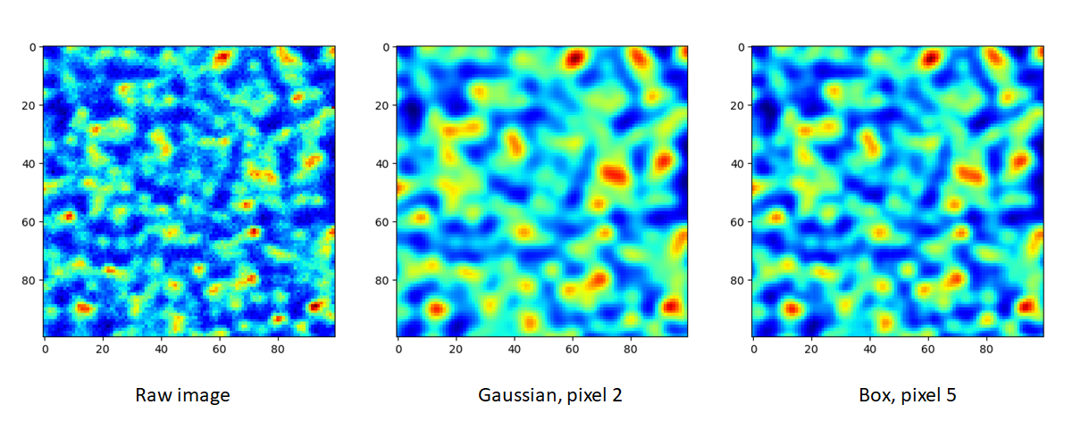
Smoothing

If the raw image quaility is very low, sometimes you need to smooth it. smooth() and smooth_multi() functions are used to smooth the raw images in the image stack. The latter is the multiprocessing version of the former. Two smoothing methods are available at present, they are Gaussian and Box, respectively. If the meth is Gaussian, a Gaussian function will be used for the smoothing, the parameter of pixel determines the sigma of the Gaussian function. If the meth is Box, a \(n \times n\) matrix is used to convolve the raw image, each element in the matrix equals to \(1/n^2\). Likewise, the parameter of pixel is used to determine \(n\). The following images show how the smoothing will look like.

To do the smoothing, you need to call the following function with parameters meth and pixel:

imstack.smooth(meth='Gaussian', pixel=2, verbos=False)

Fliping the images

Sometimes you need to flip the images in the dataset to match the reference image, such as to measure a planar mirror using XSS technique with reference beam.

An attribute flip is used to tell the codes how to flip the image. The default value is None. The acceptable values are x or y.

If

imstack.flip = 'x'

The raw images in the dataset will flip in the horizontal direction when read_data() function is called.

Otherwise,

imstack.flip = 'y'

The raw images in the dataset will flip in the vertical direction when read_data() function is called.

On the left is the raw image. In the middle is the image flipped horizontally, Imagestack.flip=’x’. On the right is the image flipped vertically, Imagestack.flip=’y’.

You can also directly call flipstack() method once the above attribute has been set:

imstack.flipstack()

Rotating the images

In some cases, you need to rotate the raw images for some degrees, such as in the example of plane mirror measurement with reference beam.

Two methods are provided to do the rotation. One is to rotate the raw images 90 degrees counterclockwise. The method name is rot90deg(). To call this method:

imstack.rot90deg()

On the left is the raw image, on the right is the rotated image. The rotation is 90 degrees counterclockwise.

Another method is rotate().

imstack.rotate(45)      # In [deg]

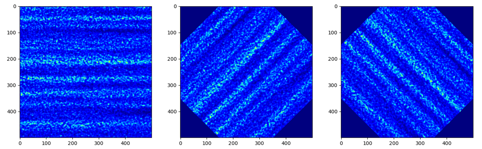
On the left is the raw image. In the middle is the image ratated with +45 degrees. On the right is the image rotated with -45 degrees.

Detector pixel size determination

To determine the detector pixel size, we scan the diffuser in one direction with a relatively large step at first, 10 um for example. The speckle pattern will move according to the scan. If the scan direction is along the x-axis, the speckle pattern will move along the x-axis too.

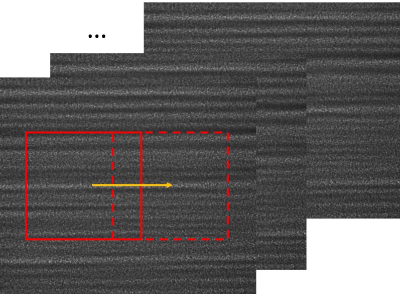
We choose a subregion from each image to track the speckle pattern movement using cross-correlation. The tracked moving is in the unit of pixels. All the images extracted from the subregion are compared with the first raw image. Thus, the tracked speckle pattern shifts will be along a straight line. We fit the tracked shifts into a straight line, and the pixel size is calculated by 1 over the slope of the fitted line.

Note

The subregion set in this function is related to the cropped image stack. That is to say, if we have set ROI for the image stack, then the subROI parameter is the coordinate to the newly cropped images by ROI, NOT to the raw images.

If display is True, the fitting results will be shown.

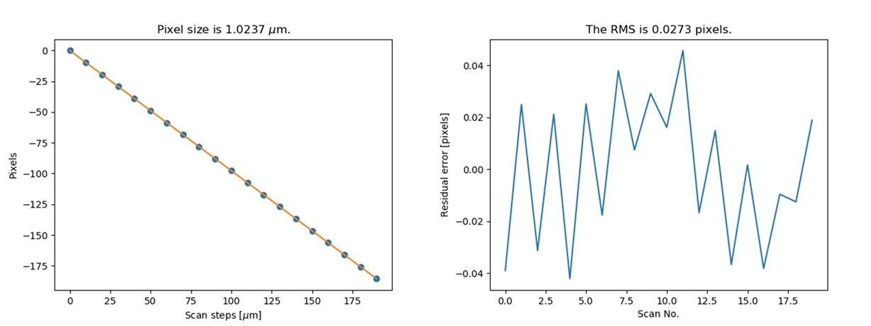
The fitting results and the residuals.

Please refer to the Tutorial for the use of this method.

The speckle-based techniques included in Tracking class

Note

In this package, we assume the incident beam is from the quasi-parallel beam from the synchrotron radiation source going through the beamline without any other optics except one monochrometer. If the incident is a quasi-spherical wave, some modifications are needed for some techniques.

Should mention upstream and Downstream problem!!! ……

The Tracking class is the container for the various speckle-based techniques. At least one image stack is needed as the input of the Tracking class. These image stacks are defined as the Imagestack classes. There are up to 4 image stacks needed according to the different data processing modes. The following list shows the number of image stacks needed for different modes. Each row has the same scan dimension scandim for each technique, each column represnts a specific type of the technique.

imstack1, imstack2, imstack3, imstack4 represent the Imagestack class needed for each tracking mode.

Scan dimension	XSS self	XST self [2]	XSS with references	XST with reference [4]	XSVT with reference
x	imstack1(x sam)	imstack1(x sam1), 2(x sam2)	imstack1(x sam), 2(x ref)	-	-
y	imstack1(y sam)	imsatck1(y sam1), 2(y sam2)	imstack1(y sam), 2(y ref)	-	-
xy [1]	-	imstack1(x sam1), 2(x sam2), 3(y sam1), 4(y sam2) [3]	imstack1(x sam), 2(x ref), 3(y sam), 4(y ref)	-	-
random	-	-	-	imstack1(sam), 2(ref)	imstack1(sam), 2(ref)

[1]

The scandim set to ‘xy’ is exclusively used for ‘2D’ data processing, it is valid only when Tracking.dimension is ‘2D’.

[2]

For XST techniques (self or with reference), there will be only one image in each image stacks.

[3]

For self-reference XST technique, it is possible that imsatck1 and imstack3 are identical.

[4]

The scandim is not valid and not used in XST technique with reference beam.

The implementation of each of these tracking modes used in this package will be introduced in this section. For the explanation of the physics and theory of these tracking modes please refer to The speckle-based wavefront sensing techniques.

As to the practical implementation of these techniques within this python package, two essential methods are XSS_withrefer() and XST_self(), as well as their multiprocessing form of XSS_withrefer_multi() and XST_self_multi(). They represent the XSS technhique with reference beam and Self-reference XST technique, respectively. Other methods are based upon these two methods.

Apart from the above mentioned speckle-based techniques, the Tracking class has provided other auxiliary functions. They are also described in the following.

Stability checking using speckle patterns

The stability() method defined in the Tracking class is used for the stability checking.

To do stability checking, the reference image is the first image in the image folder. The rest images are all compared with this reference image. This tracking mode calls the Imagematch() function directly.

Thus, before tracking, the template image will be cut according to the edge_x and edge_y.

If delayX and delayY are the tracked results, the real shifts should be delayX - edge_x[0] and delayY - edge_y[0].

Refer to Tutorial for the use of this method. The multiprocessing mode of this method named as stability_multi() is also implemented.

Reference and sample image stacks collimating before tracking

There are some occasions that you need to collimate the speckle pattrns from two image stacks before you do any speckle tracking. It is needed particularly when the tested optic is a planar reflecting mirror and we have another incident beam image stack for reference. The collimate() function is designed for such situation.

In order to use collimate() function, two image stacks Imagestack need to be defined and as the input of the Tracking class.

We use the first image from the two image stacks to do the collimation. Similar to the stability check, we cut one image in the first image stack according to edge_x and edge_y. Usually a very large area is cropped for collimating. We still invoke the Imagematch() fucntion to cross-correlate the two images from two different image stacks. Finally, we move all the images in the two image stacks according to the obtained speckle pattern shifts. After calling this method, all the images in the two image stacks will be aligned.

The following images show that before the collimation, two images from the different image stacks are not aligned well.

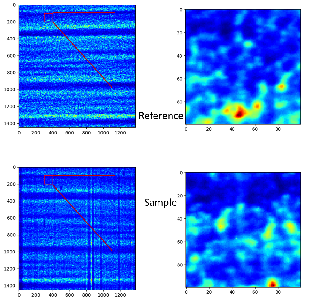
Then we do the collimating.

from spexwavepy.trackfun import Tracking

track = Tracking(imstack_sam, imstack_ref)
track.collimate(150, 250)

Where in the above code block, imstack_sam and imsatck_ref are two Imagestack classes. They represent the loaded reference and sample image stacks, respectively.

After we invoke the collimate() method, the two images from the reference and sample image stack are well aligned, as shown in the following images.

Please refer to the example Plane mirror measurement with reference beam for the use of collimate() function in real data processing procedure.

XSS technique with reference beam

The XSS_withrefer() function and XSS_withrefer_multi() function are used to process the scanned data. In this method, a reference image stack is needed. Please refer to XSS technique with reference beam for the detailed description of the physics of this technique.

The important parameters of these two functions are edge_x, edge_y, edge_z, hw_xy, pad_xy. The last two parameters, hw_xy and pad_xy are only important in 2D case.

edge_x, edge_y and edge_z defines how the raw template images are cut. If the scan is along ‘x’ direction, scandim = ‘x’, edge_x is useless. Likewise, if scan is along ‘y’ direction, scandim = ‘y’, edge_y is useless.

The diffuser was scanned along the y or x direction. At each scan position, an image was taken.

For 1D case, only a small strip of data from each raw image is extracted. As a result, the whole image stack is cropped. This is done by setting ROI for the image stacks.

The cropped data strip for 1D data processing in y scan direction.

The cropped data strip for 1D data processing in x scan direction.

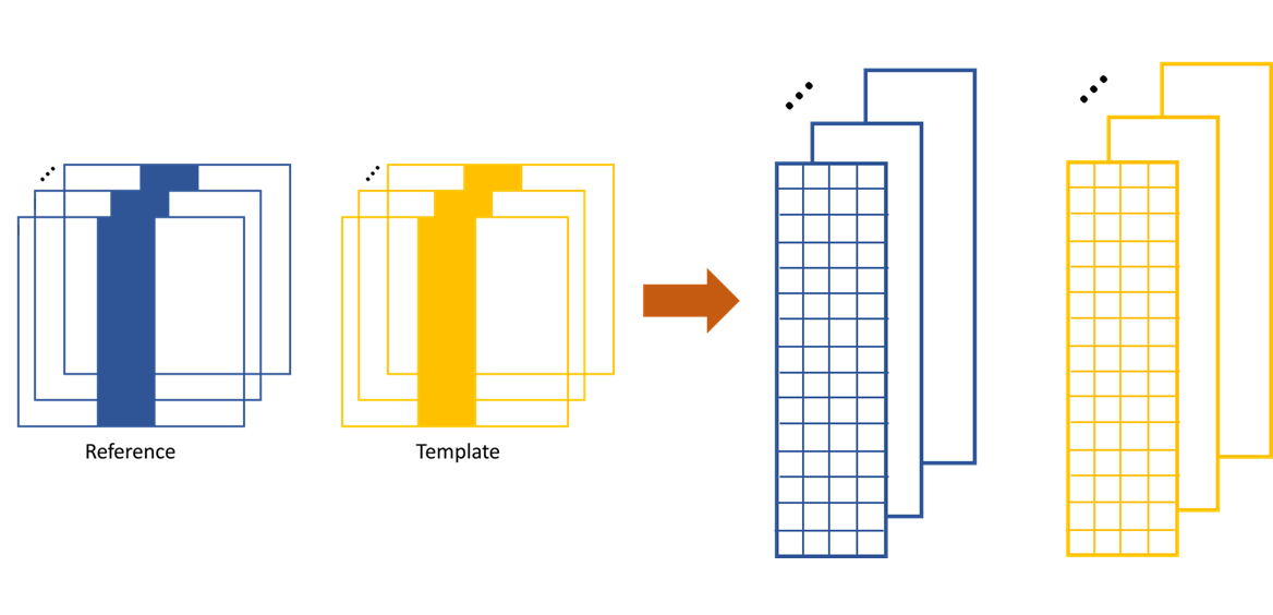
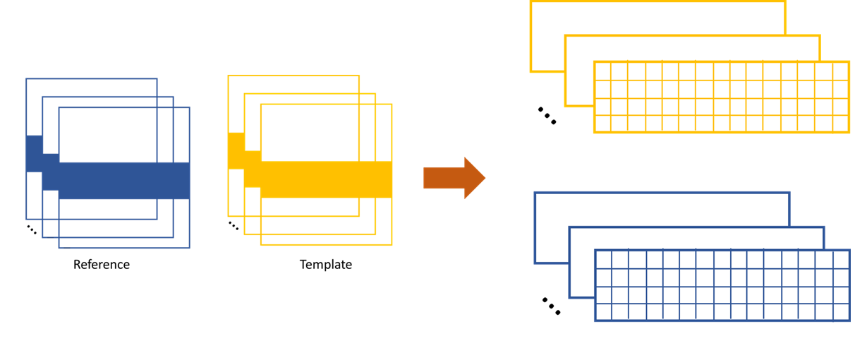
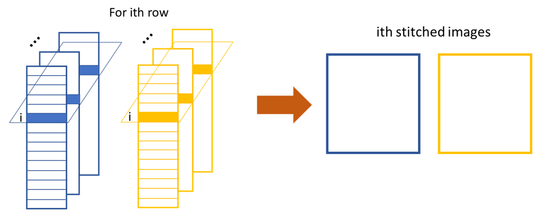
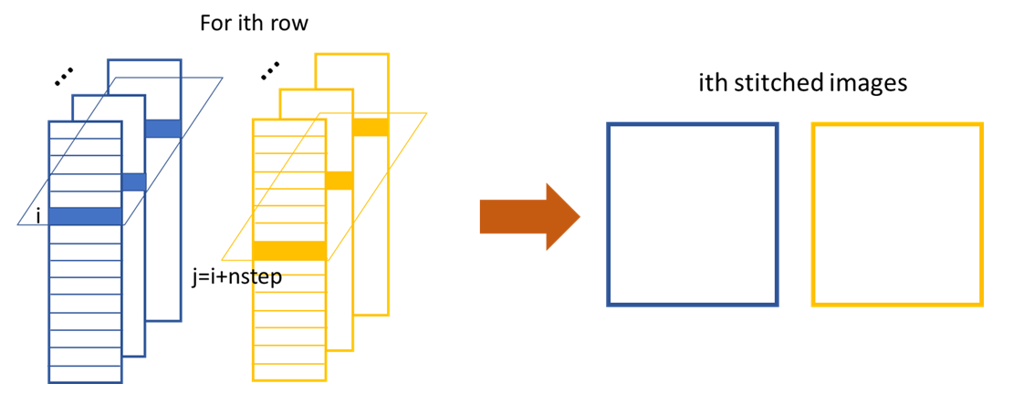
The XSS technique then process the data row(column) by row(column). Each raw image in the image stack are taken at different diffuser position. If we extract the ith row/column of every raw images and then stitch them together, a new image is generated. Two images will be generated from both reference image stack and the image stack with test optic.

The stiched images for y scan data.

The stiched images for x scan data.

The newly generated two images are cross-correlated to track the speckle pattern shifts. As mentioned in the above, edge_x is used for the y scan data. It is not used for the x scan data. On the contrary, edge_y is used for the x scan data, not used for the y scan data. edge_z are used for both data set. z is the direction representing the scan number.

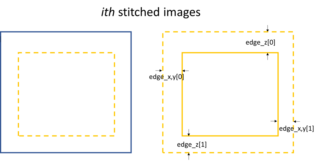
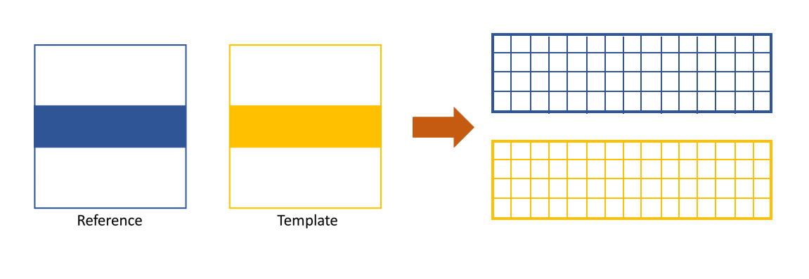
Stiched image for 1D data processing.

Loop over each row in the raw image stack, a 1D speckle shift will be obtained.

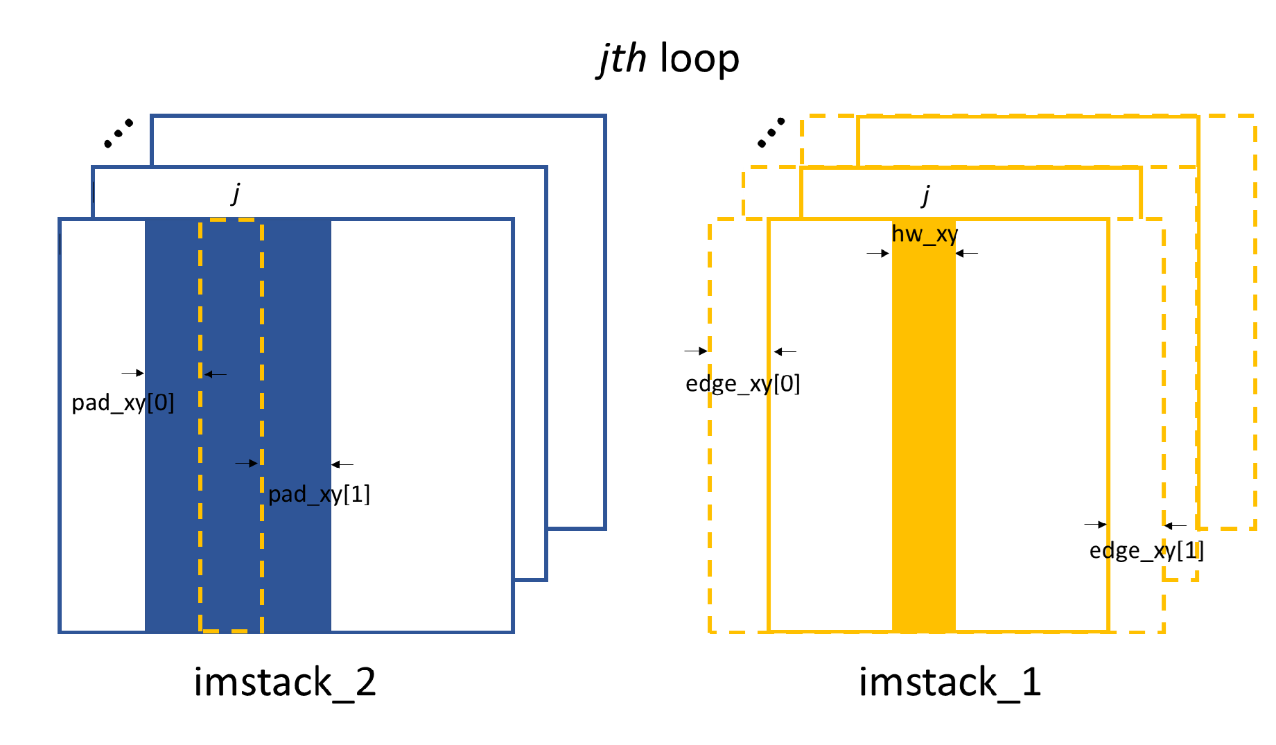
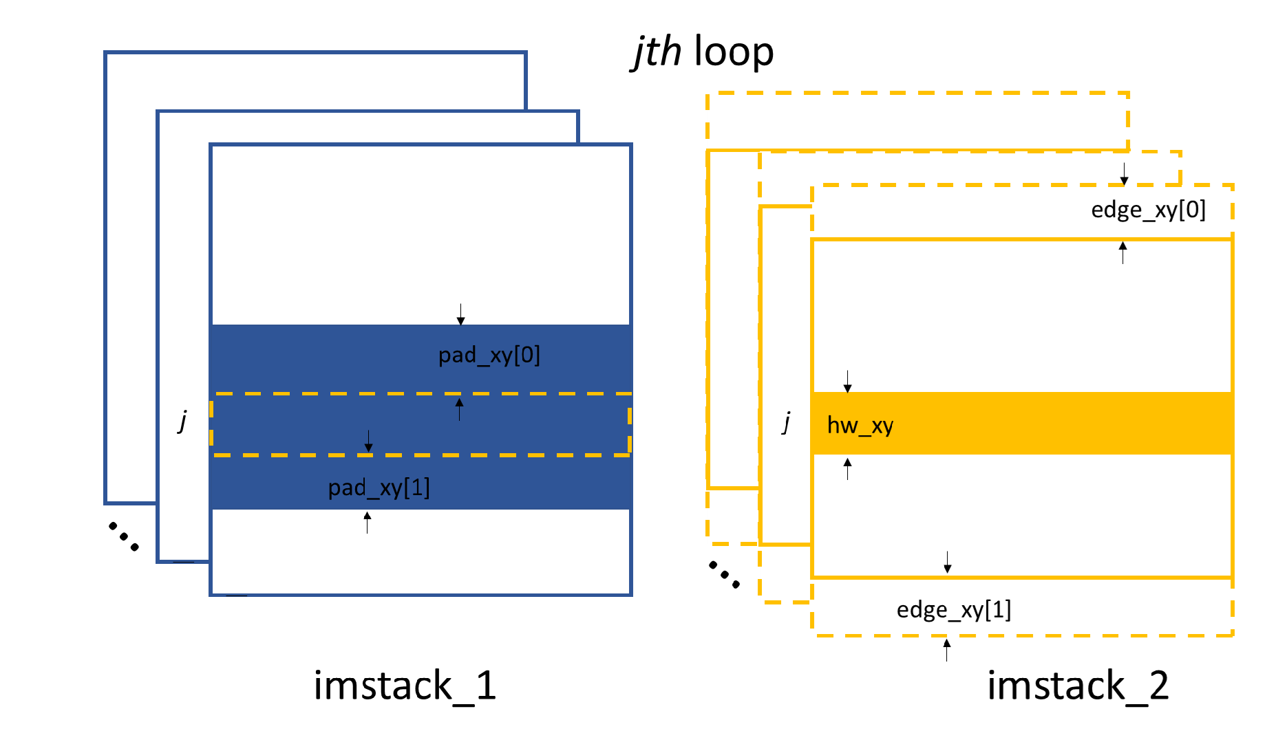
For 2D case, the similar 1D data processing procedure described in the above will be looped over the horizontal or vertical direction. For y scan direction, the outmost layer of the loop is along the x direction, as shown in the following picture. The obtained speckle pattern shift is the 2D shift along the the y direction.

The loop is over x direction when the scan is along y direction.

Likewise, if the scan direction is x, the outmost loop of the 2D data processing will be along the y direction. The obtained speckle pattern shift is in the 2D shift along the x direction.

The loop is over y direction when the scan is along x direction.

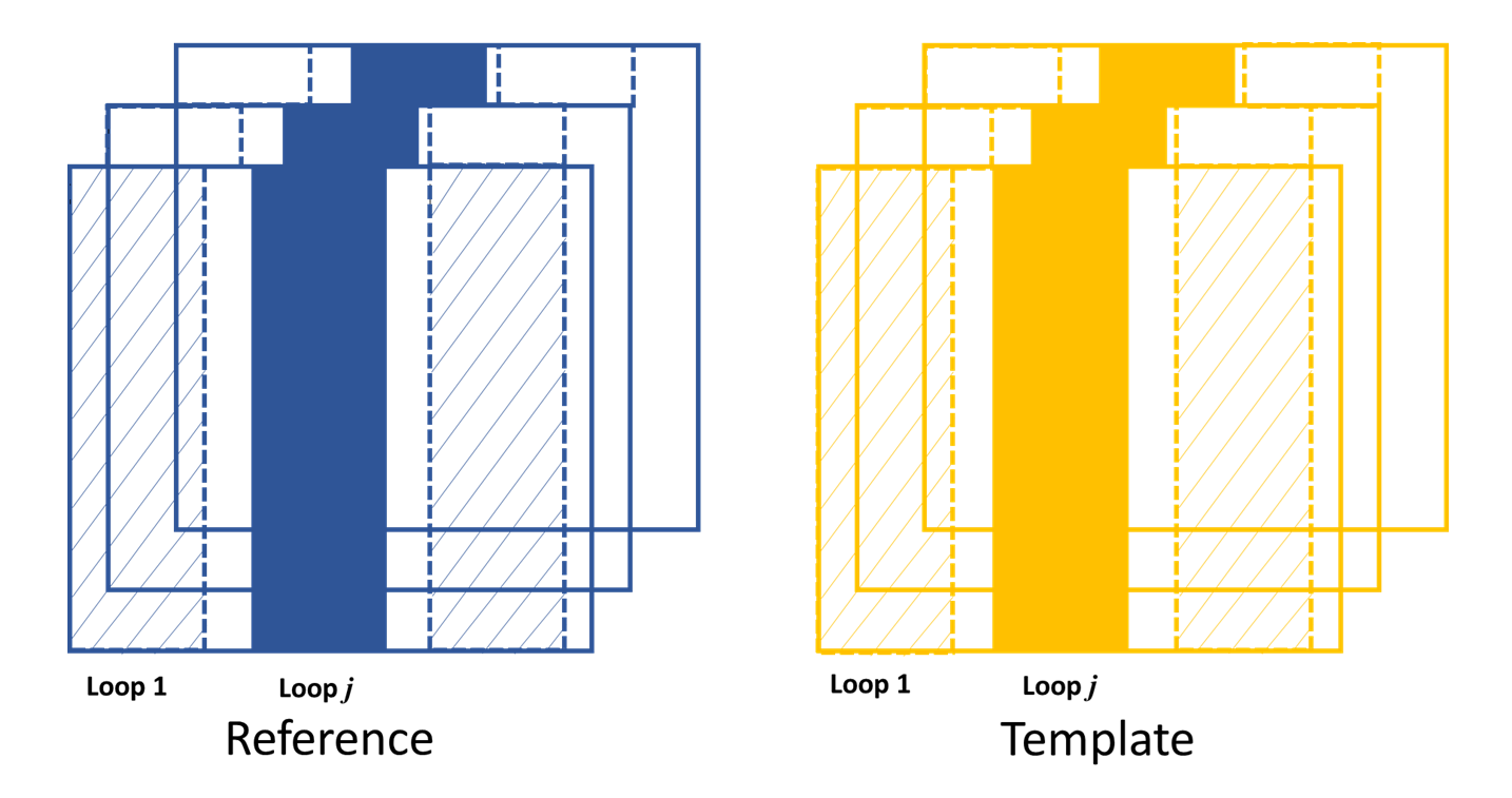
According to the above description, two more parameters play important roles. As in the 1D case, edge_x, edge_y and edge_z define how to cut the raw images in the image stack. hw_xy defines the width / height of the subregion for the 2D data processing if the scandim is ‘y’ / ‘x’. Each subregion is a strip of data resembles that in 1D case. The subregion will move to cover the whole range of the raw images. We use hw_xy to define the width / height of the window, i.e., the stitched image, to be coross-correlated during each loop. The reference stitched image should be larger than the template, we use pad_xy to define how larger the reference stitched image is. Apparently, pad_xy[0] and pad_xy[1] should be smaller or equal to edge_x(edge_y)[0] and edge_x(edge_y)[1], respectively. The larger the pad_xy is, the more trackable the image is, the slower the tracking process can be.

2D image processing for y scan data.

2D image processing for x scan data.

The remaing operations are the same as the 1D case described in the above.

Note

Note that in order to do the integration to reconstruct the wavefront, if scandim is ‘xy’, the 2D results in two directions will be cut to the same size automatically.

As been described in the XSS technique with reference beam section, by tracking the speckle patter shifts, we can obtain the slope of the wavefront from this techinque. Thus, the sloX and/or sloY are stored in the Tracking class due to the scan direction. The related postprocess fucntions are slope_pixel() and slope_scan(). Please refere to Slope reconstruction in the Post processing of the tracked speckle pattern shifts section for more description of the algorithms.

Self-reference XSS technique

The XSS_self() function and XSS_self_multi() function are used for the self-reference XSS technique. In terms of speckle pattern tracking, they are only a special case of XSS technique with reference beam. We only need to be careful that for this technique, usually only one image stack is provided for the Tracking class.

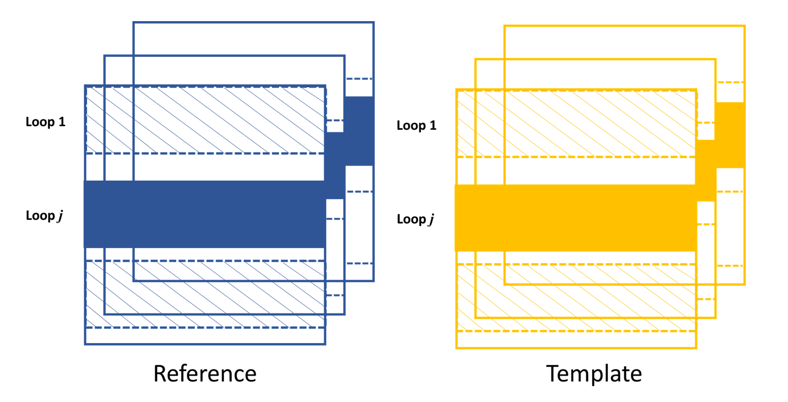
Since it is a self-reference scheme, the template image stack and the reference image stack are the same one. Slightly differ from XSS technique with reference beam, the generated stiched images are from different (i th and j th) rows/columns extracted from the same raw images in the stack.

The generation of stiched images from two seperate rows of the raw images within the image stack.

Apart from the newly introduced nstep parameter, all the other parameters are the same as in the corresponding XSS_withrefer() and XSS_withrefer_multi() functions, as already been described in the above.

However, the physical quantities directly reconstructed from this technique are dfferent from the XSS technique with reference beam. They are the local curvatures of the wavefront. Please refer to self-reference XSS technique for detailed physics.

As a result, only curvX or curvY are stored in the Tracking class. The related postprocess fucntion is curv_scan(). Please refer to Local radius of curvature reconstruction section for details.

Self-reference XST technique

Function XST_self() and its multiprocessing version XST_self_multi() is used for the self-reference XST technique.

Unlike the scan-based techniques, XST techinque only requires two images. Each image is taken when the diffuser is at one position. The diffuser can be moved vertically or horizontally, as long as the step of the movement is known. Each image constitutes the image stack.

For more of the principle of this technique, please refer to Self-reference X-ray Speckle Tracking (XST) technique. We only elaberate the implementation of this technique here.

For 1D case, like the scan-based techniques, a stripe of data along the x or y direction is extracted, depending on the scandim. The data strip needed is set by ROI.

The cropped data strip for 1D data processing in x direction, Tracking.scadim is ‘x’. The strip of the image is extracted according to the ROI.

The cropped data strip for 1D data processing in y direction, Tracking.scadim is ‘y’. The strip of the image is extracted according to the ROI.

There are some important parameters needed for the implementation of this technique. Those parameters are edge_x, edge_y, hw_xy, pad_x and pad_y.

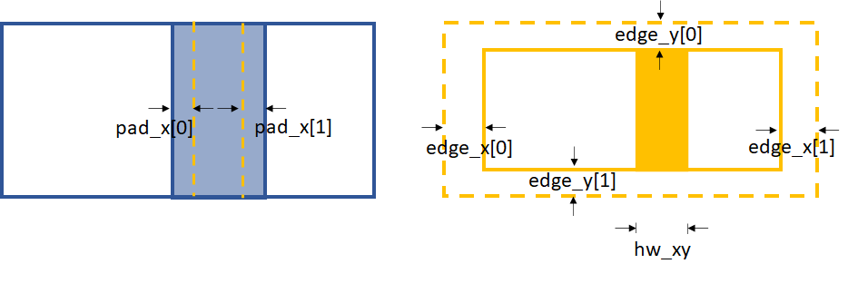
Parameters for 1D data processing in x direction

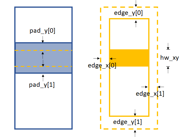
Parameters for 1D data processing in y direction

edge_x and edge_y define the area to be cut from the template in order to be able to do the cross-correlation. Unlike the XSS technique, we need hw_xy to generate the subregion from the template for cross-correlation. Besides, pad_x or pad_y is also needed depending on the scandim.

If the scandim is ‘x’, then hw_xy is the width you want to choose for the generated subregion, pad_x defines the extra area in the reference image that is needed to do the cross-correlation, pad_y is useless in this case; if the scandim is ‘y’, hw_xy is the height you want to choose for your subregion, pad_y defines the extra area needed in the reference image, pad_x is useless in this case.

Repeat the above procedure horizontally (scandim is ‘x’) or vertically (scandim is ‘y’) for the whole extracted subimage, a 1D speckle shift will be obtained.

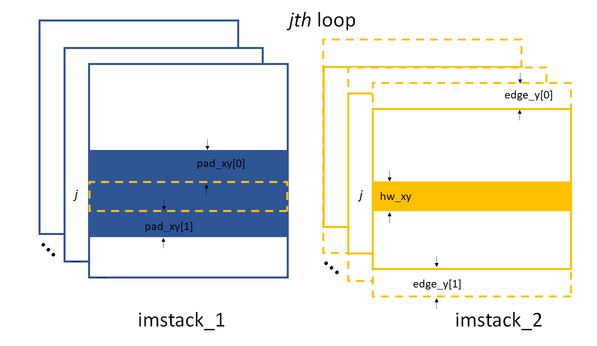
For 2D case, the above procedure for 1D shift will be repeated horizontally or vertically for the whole image, depending on the scandim. If the scandim is ‘x’, the 1D procedure will be repeated vertically. Otherwise, the 1D procedure will be repeated horizontally.

There are several more parameters needed apart from those in the 1D case. Also, some parameters are slightly different compared to the 1D case.

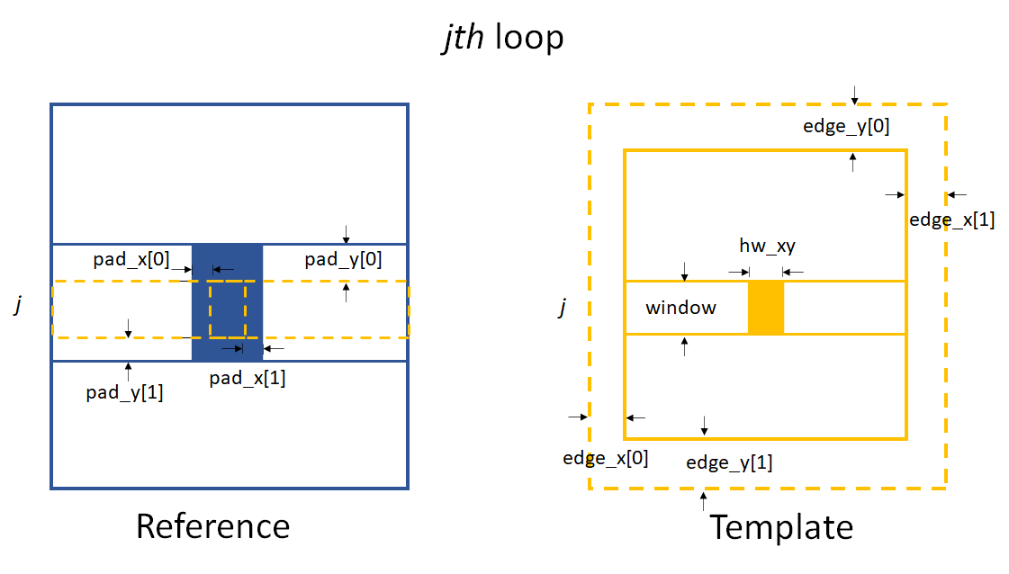
Parameters for 2D data processing when Tracking.scandim is ‘x’.

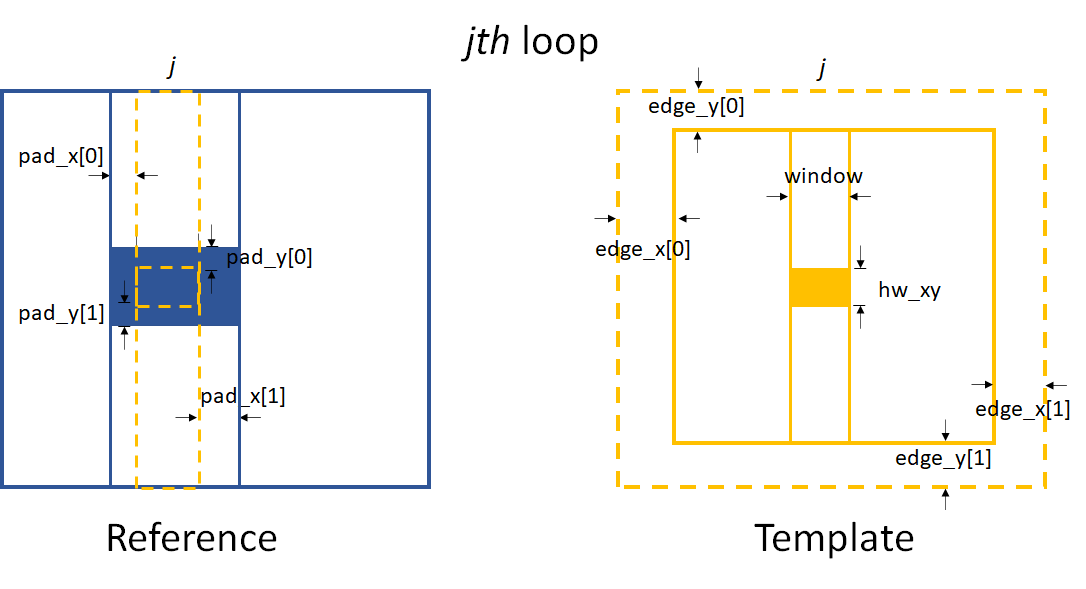
Parameters for 2D data processing when Tracking.scandim is ‘y’.

As shown in the above images, edge_x and edge_y define the cutting areas for the raw template image. Then window and hw_xy define the real size of the subregion used for tracking. If the scandim is ‘y’, window is the width of the subregion, hw_xy is the height of it; if scandim is ‘x’, window is the height of the subregion and hw_xy is the width of it. pad_x and pad_y determines the extra area for tracking.

At each loop, we do the 1D data processing procedure. The whole loop will cover the full area of the image.

Note

If scandim is ‘xy’, then edge_x and edge_y should be the same, as well as the elements within them. So is the pad_x and pad_y.

We can calculate the wavefront local curvature from the obtained speckle tracking shifts, according to the principle of the self-reference XST technique. As a result, only curvX or curvY are stored in the Tracking class. The related postprocess fucntion is curv_XST(). See Local curvature reconstruction for more details.

Conventional XST technique with reference beam

Function XST_withrefer() and its multiprocessing form XST_withrefer_multi() are the two functions used for the data processing of the Conventional XST technique. Two image stacks should be provided for this method. Each image stack has only one image. The fisrt image stack consists one image when the diffuser is in the beam. The second image stack consists one reference image without the tested optical elements.

All the parameters for XST_withrefer() and XST_withrefer_multi() are the same as the Self-reference XST technique which have been described in the above.

However, unlike the Self-reference XST technique, the physical quantities directly reconstructed from this technique are local curvatures of the wavefront. They are stored in the parameters curvX and/or curvY in the Tracking class. The related postprocess fucntion is curv_XST(). Please refer to Local radius of curvature reconstruction section for the details.

XSVT technique

XSVT_withrefer() and its multiprocessing form XSVT_withrefer_multi() are two functions used for the data processing of the XSVT technique. Since this type of technique needs images of the reference beam and the beam with tested optics, so we need two image stacks. Each image in the image stacks are taken at one random scan position of the diffuser during the movement. As a result, the scandim of the Tracking class is set to be ‘random’, the scanstep is useless.

Like the XSS-type techniques, the raw image stack is a 3D data set. Unlike the XSS-type techniques, the scan step in this technique has no clear physical meaning. Also, the ‘1D’ mode is NOT supported in this technique. The data processing mode in this technique is assumed to be two-dimensional.

Similar to the XSS-type techniques, the XSVT technique will process the data row by row and column by column to obtain the displacements in two dimensions. Since there is no clear physcial meaning in the scan direction, we obtain the speckle pattern shifts in x direction from the row-by-row data processing and in y direction from the column-by-column data processing. As a result, the obtained shifts are in the unit of the pixels size rather than the scan step as in the XSS-type techniques.

Due to the above reasons, for the practical implementation of the XSVT technique, we do the speckle tracking data processing two times to obtain the shifts in x and y direction, respectively. The data processing procedure resembles the 2D case XSS technique with reference beam.

To obtain the speckle pattern shift in the x direction, the outmost loop is along the same direction.

The loop is over x direction to obtain the speckle pattern shift in this direction.

Likewise, the outmost loop is along y direction if the speckle pattern shift in y direction is to be tracked.

The loop is over y direction to obtain the speckle pattern shift in this direction.

Although the implementation of the codes are almost the same as the XSS technique with reference beam, the shifts obtained from XSVT technique are in the unit of pixel size rather than the scan step as from the XSS-type techniques.

The important parameters of these two functions are edge_xy, edge_z, hw_xy, pad_xy.

2D image processing to obtain shifts in x direction. The chosen strip belongs to the 1D processing procedure within each loop.

2D image processing to obtain shifts in y direction. The chosen strip belongs to the 1D processing procedure within each loop.

hw_xy defines the window size of the subregion to be processed on the raw image. For XSVT technique, we will do the speckle tracking in both x and y direction, thus, hw_xy is the same for these two cases. edge_xy defines the edge to be cut on the template images, they are the same for both x and y directions.

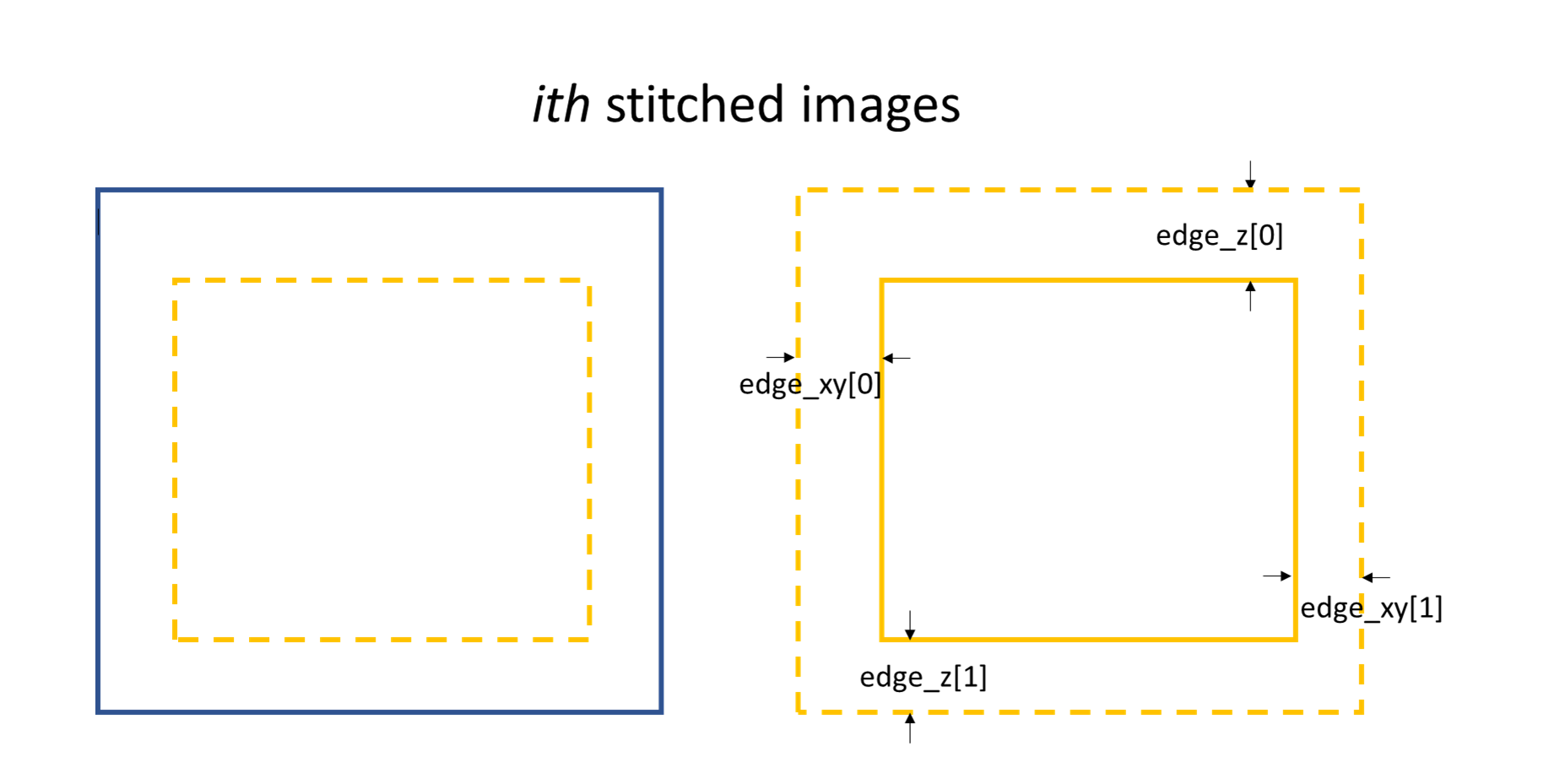
Stiched images for speckle tracking.

Within every loop, the strip data in one image stack will be stiched together to obtain the image for speckle tracking. edge_z defines the edge to be cut on the stiched template image in the scan direction, as shown in the above. The remaining procedure is the same as in the XSS technique with reference beam

Refer to the principle of the XSVT technique, the physical quantities directly reconstructed from this technique are the wavefront slopes in x and y directions. They are stored in the sloX and sloY attribute in the Tracking class. They are reconstructed using the postprocessing function of slope_pixel(). See Slope reconstruction for more details.

Hartmann-like data processing scheme

Hartmann_XST() is defined to mimic the Hartmann-like data processing scheme. Like the conventional XST technique with reference beam described in the above, two image stacks need to be initialized in the first place, however, each image stack consists only one image. Usually, the fisrt stack contains the image when the diffuser is in the beam, the second stack contains the reference image.

The two images are divided into many subregions. Each subregion is a rectangular box. The centre and the size of the box has been pre-defined. The cen_xmesh and cen_ymesh are the meshgrid of the x and y coordinate of the subregion centres. In addition, size[0] represents the width of the box, while size[1] represents the height. These parameters are shown in the following figure. We can use Hartmann_mesh_show() function to show the defined subregions. Please refer to Auxiliary functions for the usage of this auxiliary function.

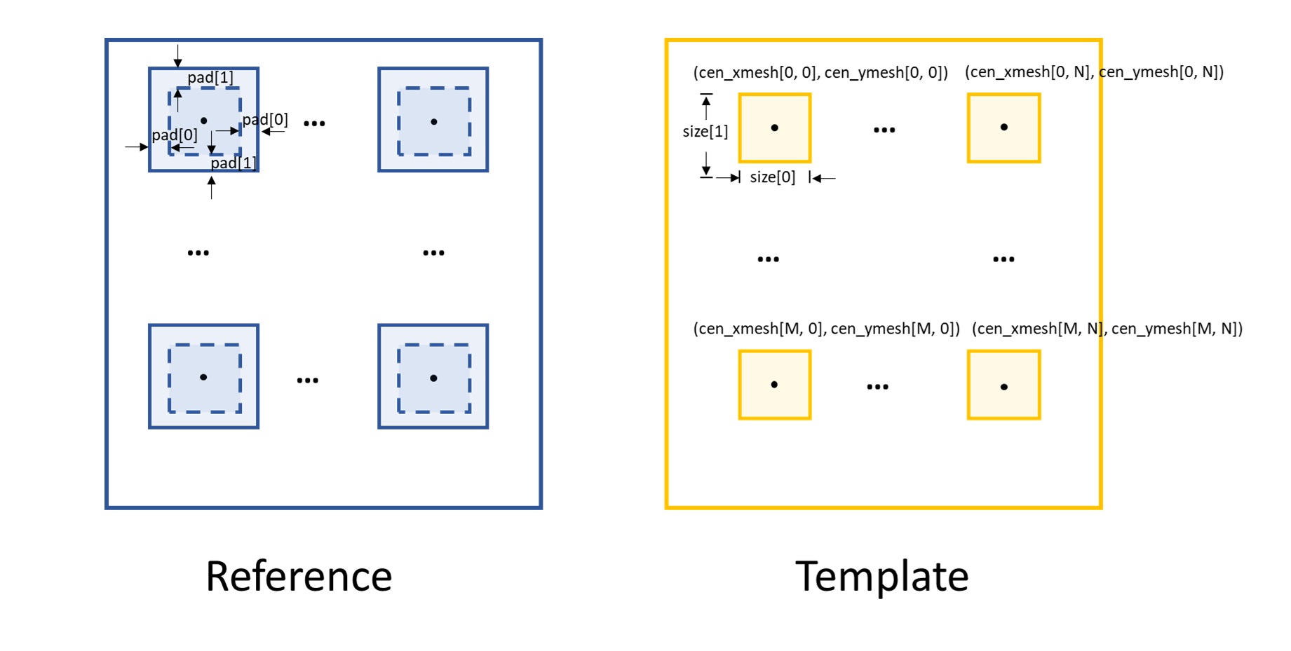
In order to do the cross-correlation for each subregion, we need to expand each box on the reference image, the parameter pad is used for this purpose. Also as shown in the figure, pad[0] relates the expansion in the x direction, pad[1] in the y direction. The cross-correlation with subpixel registration accuracy is performed by looping over the rectangular boxes.

For more usage of the Hartmann_XST() function, please refer to this example.

Note

Unlike other data processing mode, we only provide Tracking.delayX and Tracking.delayY for this method. Recovering the appropriate physical quantities (slope or curvature) from the speckle shifts is left to the discretion of the users.

Post processing of the tracked speckle pattern shifts

For various speckle tracking modes, the tracked speckle pattern shifts can represent different physical quantities. Please refer to the principle of the speckle-based wavefront sensing techniques for detailed description of the physical meanings of the shifts. The postfun module converts these shifts to the phsycial quantities according to the specific technique. We will describe the functions included in this module in the following.

Slope reconstruction

According to the principle of the speckle-based wavefront sensing techniques, in general, we can reconstruct the local wavefront slope from the tracked shifts if the reference beam is existed. Two functions, slope_scan() and slope_pixel(), are provided in the postfun module. They are called depending on which speckle tracking technique is used.

For the XSS technique with reference beam, the tracked shifts are in the unit of scan step along the scan direction, the slope_scan() function is called. If the tracked shifts are in the unit of pixel size, such as the other direction (perpendicular to the scan direction) of the XSS technique with reference beam, both directions of the conventional XST technique and XSVT technique, the slope_pixel() function is called.

If we use \(\mu\) to represent the tracked shifts regardless of its unit, \(p\) the detector pixel size, \(s\) the scan step size, for slope_scan() function, we have:

\[slope = \frac{\mu \times s}{d}\]

for slope_pixel() function, we have:

\[slope = \frac{\mu \times p}{d}\]

In the above two equations, \(d\) represents the distance. If the diffuser is placed in the downstream of the tested optic, \(d\) is the distance betweeen the diffuser and the detector. Otherwise, if the diffuser is placed in the upstream, \(d\) is usually set to be the distance between the centre of the optic and the detector.

Local curvature reconstruction

Refer to the principle of the speckle-based wavefront sensing techniques, if there is no reference beam, usually the local radius of curvature is reconstructed from the tracked speckle pattern shifts. Similar to the functions for the local wavefront slope reconstruction, two functions are also provided to reconstruct local wavefront curvature depending on the specific speckle tracking technique. They are curv_scan() and curv_XST(), respectively. They both return the local curvature of the wavefront at the detector plane. It is easy to convert this to the wavefront curvature at the diffuser plane.

The curv_scan() function is used by Tracking class for the self-reference XSS technique, while the curv_XST() function is used by the same class for the self-reference XST technique.

Similar to the local wavefront slope reconstruction, we use \(d\) to represent the distance used for the local wavefront curvature reconstruction. Two situations need to be distingushed. If the diffuser is placed in the downstream of the tested optic, \(d\) is the distance betweeen the diffuser and the detector. Otherwise, if the diffuser is placed in the upstream, \(d\) is usually set to be the distance between the centre of the optic and the detector.

We show the downstream case at first.

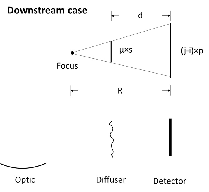
The downstream case.

If we use \(p\) to represent the detector pixel size, \(\mu\) the tracked shift, \(s\) the scan step size, \(j-i\) the spacing of the columns/rows to be extracted and stiched, \(m\) the magnification factor, then we have the following equations.

For self-reference XSS technique (curv_scan()):

\[m = \frac{\mu \times s}{(j-i) \times p} = \frac{R-d}{R}\]

For self-reference XST technique (curv_XST()):

\[m = \frac{s}{\mu \times p} = \frac{R-d}{R}\]

The local curvature of the wavefront at the detector plane is \(1/R\), thus we have:

\[\frac{1}{R} = \frac{1-m}{d}\]

Now let’s look at the upstream case.

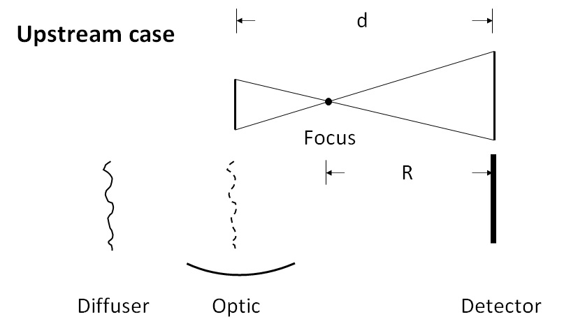
The upstream case.

We use the same symbols to represent the related physical quantity. For the upstream case, the distance betweeen the diffuser and the detector is assumed to be the centre of the tested optic and the detector, since we assume the incident beam has negligible divergence and the beam is modulated only after the optic.

The equation to describe the geometric relation is slightly different from the downstream case.

For self-reference XSS technique (curv_scan()):

\[m = \frac{\mu \times s}{(j-i) \times p} = \frac{d-R}{R}\]

For self-reference XST technique (curv_XST()):

\[m = \frac{s}{\mu \times p} = \frac{d-R}{R}\]

The local curvature of the wavefront at the detector plane is:

\[\frac{1}{R} = \frac{1+m}{d}\]

Warning

Apart from the above two cases, there are other geometric situations. However, these other situations can be equivalent to the the above two cases, only need to note that the obtained curvature may no longer at the detector plane, it may at the diffuser plane instead. For plane mirror, set mempos to downstream is usually better since its focus is always very far.

2D integration for post processing

We also provide functions to do the 2D integration from the gradients in x and y directions. These functions are useful when reconstructing the wavefront from the local wavefront slope and in some other situations. Two functions, Integration2D_SCS() and Integration2D_FC(), are provided to do the 2D integration in this package.

The detailed mathematics of the SCS method can be found from [SCSmeth], the FC method from [FCmeth].

These two functions can be called once the local wavefront slope in two directions are obtained. The wavefront slope information is stored in sloX and sloY of the Tracking class.

The function is invoked as:

from spexwavepy.postfun import Integration2D_SCS, Integration2D_FC
surface = Integration2D_SCS(Tracking.sloX, Tracking.sloY)

or

surface = Integration2D_FC(Tracking.sloX, Tracking.sloY)

Please refer to Tutorial for the use of 2D integration to obtain the wavrfront.

[SCSmeth]

Simchony T, Chellappa R, Shao, M. Direct analytical methods for solving Poisson equations in computer vision problems IEEE transactions on pattern analysis and machine intelligence 1990, 12(5), 435-446. https://doi.org/10.1109/34.55103

[FCmeth]

Frankot, R, & Chellappa, R. A method for enforcing integrability in shape from shading algorithms IEEE Transactions on pattern analysis and machine intelligence, 1998, 10(4), 439-451. https://doi.org/10.1109/34.3909

Auxiliary functions

EllipseSlope() function is an auxiliary function used to calculate the slope error for an elliptical mirror with known parameters. This function is used to calculate the slope error on the mirror surface through an iterative algorithm. Please see the Mirror slope error curve (1D) reconstructed from the dowmstream setup example for the usage of this function.