Examples

Warning

Due to the different behaviours of the Python built-in multiprocessing module on Linux and Windows operating systems, the current version of spexwavepy can only run on Linux machine for the multiprocessing version of each technique. Future work will extend this package to run on multicores for the Windows system.

Apart from the sample codes shown for the tutorial, we also provide several examples in spexwavepy package to help users to learn how to do the data processing for different speckle-based techniques. All the examples shown here are extracted from our previous published research papers. We also shared the raw data for users of spexwavepy package. Please refer to Getting started page for downloading these raw data.

Note

The shared raw data is only used for study. Please do not distribute the raw data. If you would like to use these raw data for publication and so on, please contact the authors of this package.

Note

To be able to run all the provided examples with shared experiment data, please change the default data folder path to where your data is stored once you download it.

Plane mirror measurement with reference beam

Note

Please find the example code from /spexwavepy/examples/planemirror_2D.py

In this example, we would like to show that how to use the XSS technique with reference beam to measure a plane mirror.

This example basically extracts from [HuXSSJSRpaper].

After detemining the data folder path and appropriate ROI for both sample and reference images, we define the Imagestack classes to contain the data. Then we define the Tracking class.

imstack_sam = Imagestack(sam_folder, ROI_sam)
imstack_ref = Imagestack(ref_folder, ROI_ref)
imstack_ref.flip = 'x'

track_XSS = Tracking(imstack_sam, imstack_ref)
track_XSS.dimension = '2D'
track_XSS.scandim = 'x'
track_XSS.dist = 833.     # [mm]
track_XSS.scanstep = 1.0  # [um]
track_XSS.pixsize = 1.07  # [um]

Note that we set flip attribute to the reference image stack. This is due to the fact that the reflected images after a mirror flipped the incident beam. So, in order to be able to track the shift of speckle patterns, we flip the reference images in the reference image stack.

We only did x scan in this example, so the scandim of the Tracking class is ‘x’. We do 2D data analysis, the dimension is set to be ‘2D’.

Before we do the speckle pattern tracking, another thing we need to do is to align the speckle patterns from the two image stacks. It is particularly needed when the test optic is a mirror. We use collimate() function to do the alignment. Please refer to the User guide for the detailed description of this function.

track_XSS.collimate(10, 200)

After that, the speckle patterns from both image stacks are aligned and ready to be tracked. We set the related parameters before we call the method used for speckle tracking. Please refer to the User guide for the detailed explanation of these parameters.

edge_x = 0
edge_y = 30
edge_z = [15, 30]
width = 100
pad_xy = 30

After setting the initial parameters, we use either single-core version XSS_withrefer() or multi-core version XSS_withrefer_multi() of the method to obtain the speckle pattern shifts. Since the scan direction is along ‘x’, then edge_x is 0. Also, the edge_z is not symmetrical.

track_XSS.XSS_withrefer(edge_x, edge_y, edge_z, width, pad_xy, normalize=True, display=False)

Or

track_XSS.XSS_withrefer_multi(edge_x, edge_y, edge_z, width, pad_xy, cpu_no=16, normalize=True)

Warning

Please check the available CPUs before calling XSS_withrefer_multi() method.

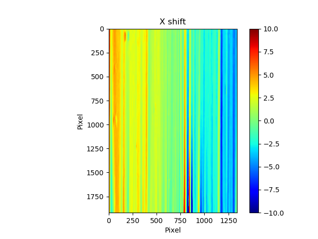
Note that we did normalization for the stiched images in this example. The shift in ‘x’ direction looks like

Since we only scanned in the horizontal (x) direction, the delayX is the only “canonical” processed data stored in the track_XSS class. No track_XSS.delayY is available. However, we do store the tracked value in another direction in the Tracking class. In this example, the shift in ‘y’ direction is stored in track_XSS._delayY.

Note

The underscored attribute such as Tracking._delayX or Tracking._delayY are not intended to be exposed to the user. However, in some cases, they do help the users with their data processing. Nonetheless, please keep in mind that the underscored data are not “canonical” basically.

It looks like

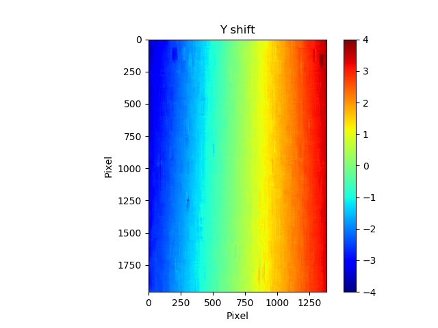
Since the tested mirror is an ultra-smooth plane mirror, the speckle shift in y direction should be very small. If we extract a central horizontal line from the 2D map of Y shift, we can see a tilted straight line

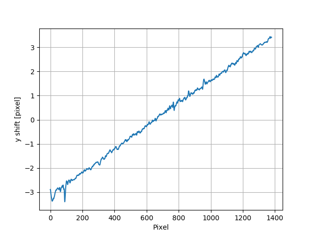
This indicate that the mirror is not perfectly parallel with the reference incident beam. The raw images need to be rotated and carefully aligned. According to the paper [HuXSSJSRpaper], the rotation angle is calculated to be around -0.275 degrees.

We can use rotate() function to do the rotation. See the User guide for its help information.

rotateang = -0.275       # [degree]
imstack_sam.rotate(rotateang)

After the rotation, the edge of the raw images is non-physical. For example, if we print out imstack_sam.data, we will see

print(imstack_sam.data)

array([[[0., 0., 0., ..., 0., 0., 0.],
     [0., 0., 0., ..., 0., 0., 0.],
     [0., 0., 0., ..., 0., 0., 0.],
     ...,
     [0., 0., 0., ..., 0., 0., 0.],
     [0., 0., 0., ..., 0., 0., 0.],
     [0., 0., 0., ..., 0., 0., 0.]],

    [[0., 0., 0., ..., 0., 0., 0.],
     [0., 0., 0., ..., 0., 0., 0.],
     [0., 0., 0., ..., 0., 0., 0.],
     ...,
     [0., 0., 0., ..., 0., 0., 0.],
     [0., 0., 0., ..., 0., 0., 0.],
     [0., 0., 0., ..., 0., 0., 0.]],

    [[0., 0., 0., ..., 0., 0., 0.],
     [0., 0., 0., ..., 0., 0., 0.],
     [0., 0., 0., ..., 0., 0., 0.],
     ...,
     [0., 0., 0., ..., 0., 0., 0.],
     [0., 0., 0., ..., 0., 0., 0.],
     [0., 0., 0., ..., 0., 0., 0.]],

    ...,

    [[0., 0., 0., ..., 0., 0., 0.],
     [0., 0., 0., ..., 0., 0., 0.],
     [0., 0., 0., ..., 0., 0., 0.],
     ...,
     [0., 0., 0., ..., 0., 0., 0.],
     [0., 0., 0., ..., 0., 0., 0.],
     [0., 0., 0., ..., 0., 0., 0.]],

    [[0., 0., 0., ..., 0., 0., 0.],
     [0., 0., 0., ..., 0., 0., 0.],
     [0., 0., 0., ..., 0., 0., 0.],
     ...,
     [0., 0., 0., ..., 0., 0., 0.],
     [0., 0., 0., ..., 0., 0., 0.],
     [0., 0., 0., ..., 0., 0., 0.]],

    [[0., 0., 0., ..., 0., 0., 0.],
     [0., 0., 0., ..., 0., 0., 0.],
     [0., 0., 0., ..., 0., 0., 0.],
     ...,
     [0., 0., 0., ..., 0., 0., 0.],
     [0., 0., 0., ..., 0., 0., 0.],
     [0., 0., 0., ..., 0., 0., 0.]]])

As a result, we need to cut the edge of the rotated images.

cut = 20
imstack_sam.data = imstack_sam.data[:,cut:-cut, cut:-cut]
imstack_ref.data = imstack_ref.data[:,cut:-cut, cut:-cut]

After that, we redefine the track_XSS class and do the same operations as before, using either single-core version XSS_withrefer() or multi-core version XSS_withrefer_multi() of the XSS tracking method, we have the following tracked shift in y direction.

We can also extract the central line

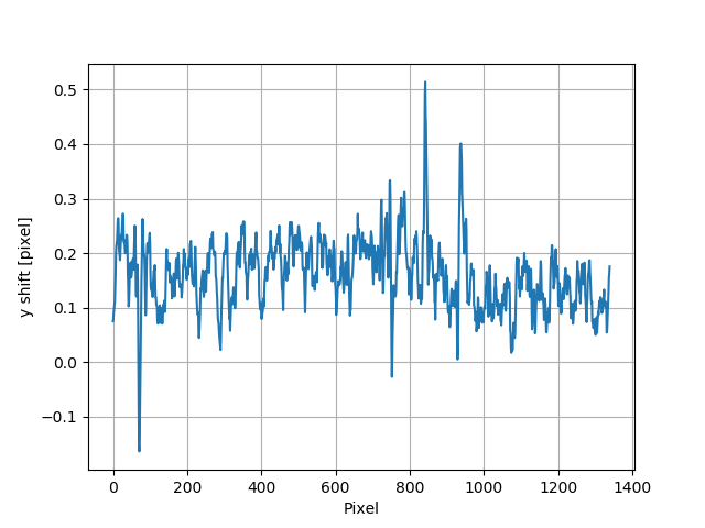
We can see the tracked speckle pattern shift in y direction has been properly corrected. We also have the tracked shift in x direction.

Besides, the slope error in x direction has also been calculated and stored in the slopeX of track_XSS class. Please refer to the principle of the XSS technique with reference beam and the User guide for reconstructing of the wavefront slope error.

[HuXSSJSRpaper] (1,2)

Hu, L., Wang, H., Fox, O., & Sawhney, K. (2022). Two-dimensional speckle technique for slope error measurements of weakly focusing reflective X-ray optics. J. Synchrotron Rad. 29(6). https://doi.org/10.1107/S160057752200916X

Measurement of the wavefront local curvature after a plane mirror

Note

Please find the example code from /spexwavepy/examples/plane_XSSself.py

In this example, we will use the self-reference XSS technique to measure the local curvature of the wavefront after a plane mirror. We will show that the fine structures appeared on the intensity image correspond to the local curvature map. This example is extracted from [HuStripeOEpaper] and [HuStripeOEpaper2]. Please refer to the papers for the detailed physics of this example.

First, let’s set the parameters for the Imagestack class imstack and the Tracking class track_XSS as usual,

ROI = [180, 1980, 690, 1270]   # [y_start, y_end, x_start, x_end]
imstack = Imagestack(folderName, ROI)
track_XSS = Tracking(imstack)
track_XSS.dimension = '2D'
track_XSS.scandim = 'x'
track_XSS.dist = 1705.0    #[mm]
track_XSS.pixsize = 3.0    #[um]
track_XSS.scanstep = 1.0    #[um]

we call XSS_self() or XSS_self_multi() function to process the data acquired using self-reference XSS technique. Please also refer to the User guide for the detailed explanation of the related parameters.

edge_x = 0
edge_y = 10
edge_z = 10
nstep = 2
width = 30
pad_xy = 10
normalize = True
#track_XSS.XSS_self(edge_x, edge_y, edge_z, nstep, width, pad_xy, normalize, display=True)
cpu_no = 16
track_XSS.XSS_self_multi(edge_x, edge_y, edge_z, nstep, width, pad_xy, cpu_no, normalize)

Warning

Please check the available CPUs before calling XSS_self_multi() method.

For this technique, the wavefront local curvature is the quantity directly reconstructed. The 2D map generated from the XSS_self() or XSS_self_multi() function is the local curvature of the wavefront on the detector plane. Since we san along the x direction, the 2D wavefront curvature is stored in the curvX attribute of Tracking class. Otherwise, the curvature in y direction is stroed in curvY. The 2D figure of the wavefront local curvature in x direction is shown below.

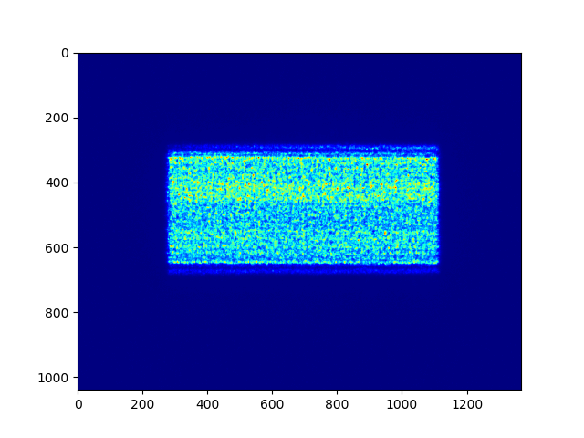
The far-field intensity images are also acquired. We read them and do the average. The image stack data are stored in the data attribute of the Imagestack class. We do the average on data. Then we show the intensity image.

import numpy as np
imstack2 = Imagestack(flatFolder, ROI)
imstack2.read_data()
ffimage = np.mean(imstack2.data, axis=0)

From the two images shown in the above, we can find that those structures in the intensity image can be related to the structures appeared in the wavefront local curvature 2D map. The two papers [HuStripeOEpaper] and [HuStripeOEpaper2] give a detailed physical explanation of this phenomenon.

[HuStripeOEpaper] (1,2)

Hu, L., Wang, H., Sutter, J., & Sawhney, K. (2021). Investigation of the stripe patterns from X-ray reflection optics. Opt. Express 29, 4270-4286. https://doi.org/10.1364/OE.417030

[HuStripeOEpaper2] (1,2)

Hu, L, Wang, H, Sutter, J. & Sawhney, K. (2023). Research on the beam structures observed from X-ray optics in the far field. Opt. Express 31(25):41000-41013. https://doi.org/10.1364/OE.499685

Mirror slope error curve (1D) reconstructed from the dowmstream setup

Note

Please find the example code from /spexwavepy/examples/curvm_XSSself.py

A curved mirror is measured in this example. The diffuser is placed downstream of the mirror.

Because the curved mirror has no available reference beam, we use the self-reference XSS technique for the measurement. It is easy to obtain the 1D curve of the wavefront curvature. This example is extracted from this paper [ZhouJSRpaper]. For the detailed description of the physics and algorithm, please refer to the paper.

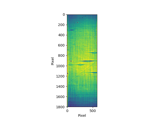
Let’s check the raw data image first.

from spexwavepy.corefun import read_one
ShowImage = True
im_sam = read_one(folderName + 'ipp_292770_1.TIF', ShowImage=ShowImage)

To obtain the 1D wavefront local curvature curve, we choose a small stripe of around 150 pixels in width, that is around 1mm wide.

ROI = [338, 643, 675, 825]          #[y_start, y_end, x_start, x_end]

imstack = Imagestack(folderName, ROI)

track_XSS = Tracking(imstack)
track_XSS.dimension = '1D'
track_XSS.scandim = 'y'
track_XSS.mempos = 'downstream'
track_XSS.dist = 1790.0    #[mm]
track_XSS.pixsize = 6.45    #[um]
track_XSS.scanstep = 0.25    #[um]

edge_x = 15
edge_y = 0
edge_z = [5, 30]
nstep = 2

track_XSS.XSS_self(edge_x, edge_y, edge_z, nstep, display=False)

After setting up the Imagestack class imstack and Tracking class track_XSS and the related parameters, we call XSS_self() function to calculate the wavefront local curvature on the detector plane. The obtained result is stored in track_XSS.curvY attribute.

In order to compare the at-wavelength measurement with the off-line NOM measurement, we need to project the wavefront on the detector plane back to the mirror surface. To do that, we need the following iterative algorithm. This algorithm has been described in detail in this paper [ZhouJSRpaper]. The main idea of the following iterative algorithm is also similar to [SebastienGrating].

Two relations are used to devise the iterative algorithm. First, the slope of the mirror can be calculated as

\[slo = \frac{1}{2}\frac{Y_{det}-y}{d-x}\]

where \(Y_{det}\) is the detector coordinate, \(d\) is the distance between the mirror and the detector plane. \(x\) and \(y\) are the mirror coordinate.

Second, the slope of the mirror is also the half of the wavefront slope. The wavefront slope can be calculated by the measured local curvature. If we integrate the mirror slope, we can have the mirror height, which is also \(y\) coordinate of the mirror.

\[y = \int_{0}^{x}slo(x)dx\]

From the above equations, the mirror slope is the measured quantity and is already known, the detector coordinate \(Y_{det}\) is also known, so is the distance \(d\).

We use the first equation to calculate the mirror surface corrdinate \(x\), the second equation to calculate \(y\). We do it iteratively. In the end, both \(x\) and \(y\) will converge.

######### Iterative algorithm for donwstream case
iy = track_XSS.delayY
loccurv_y = track_XSS.curvY
theta = 3.7e-3                     #[rad], pitch angle
mirror_L = 0.10                    #[m], mirror length
dist_mc2det = 2.925                #[m]
D = dist_mc2det + 0.5 * mirror_L * np.cos(theta)   #[m]
pixsize = track_XSS.pixsize

loccurvs = 0.5 * np.flip(loccurv_y)
detPos = np.arange(0, len(loccurvs)) * pixsize * 1.e-6     #[m]
SloErr = scipy.integrate.cumtrapz(loccurvs, detPos)           #[rad]
SloErr = np.concatenate((np.array([0.]), SloErr))                #[rad]
#Inc_corr = np.linspace(-0.5*0.08*theta/41., 0.5*0.08*theta/41, len(SloErr))
#SloErr -= Inc_corr
x_init = np.linspace(0, mirror_L, len(SloErr))                #[m]
y_init = scipy.integrate.cumtrapz(SloErr*0.+theta, x_init)             #[m]
y_init = np.concatenate((np.array([0.]), y_init))          #[m]
Y_det = y_init + 2 * (SloErr+theta) * (D-x_init)
Y_det = Y_det[0] + detPos
y_init2 = Y_det - 2 * (SloErr+theta) * (D-x_init)
x = copy.deepcopy(x_init)
y = copy.deepcopy(y_init)
for i in range(50):
    y_prev = copy.deepcopy(y)
    x_prev = copy.deepcopy(x)
    x = D - (Y_det - y) / (2 * (SloErr + theta))                   #[m]
    #sys.exit(0)
    y = scipy.integrate.cumtrapz(SloErr+theta, x)                  #[m]
    y = np.concatenate((np.array([0.]), y))                        #[m]
    y_after = copy.deepcopy(y)
    x_after = copy.deepcopy(x)
    if i>0:
        #plt.plot(x*1.e3, s*1.e6)
        print("Iteration time: " + str(i+1))
        print(np.sqrt(np.sum((y_prev-y_after)**2)))
        print(np.sqrt(np.sum((x_prev-x_after)**2)))
#########

After that, we fit the result with the elliptical mirror shape.

######### Fitting
p = 46.      #[m]
q = 0.4      #[m]
theta = 3.e-3     #[rad]
popt, pcov = scipy.optimize.curve_fit(EllipseSlope, x, SloErr, bounds=([p-1, 0., theta-0.3e-3], [p+1, 1., theta+0.3e-3]))
SloFit = EllipseSlope(x, popt[0], popt[1], popt[2])
SloRes = SloErr - SloFit
#########

We plot the measured on-line slope error and the off-line slope error together.

######### Exel data reading
import pandas

exel_folder = currentfolder + "/NOM_data.xlsx"
data_Fram = pandas.read_excel(exel_folder)
data_array = np.array(data_Fram)
x_lane1 = data_array[2:901, 1]
slo_lane1 = data_array[2:901, 2]
sloErr_lane1 = data_array[2:901, 3]
x_lane2 = data_array[2:901, 5]
slo_lane2 = data_array[2:901, 6]
sloErr_lane2 = data_array[2:901, 7]
x_lane3 = data_array[2:901, 9]
slo_lane3 = data_array[2:901, 10]
sloErr_lane3 = data_array[2:901, 11]

plt.figure()
plt.plot(x*1.e3-41, np.flip(-SloRes)*1.e6, label='At-wavelength measurement')
plt.plot(x_lane3, sloErr_lane3, label='Off-line measurement')
plt.xlabel('Mirror length [mm]')
plt.ylabel('Slope error [' + r'$\mu$' + 'rad]')
plt.legend()
#########

Note

We use the pandas library to read the xlsx file. However, the pandas library is not mandatory for spexwavepy. You can run spexwavepy well without the supoort of padans.

We can also check the fitted parameters of the elliptical mirror.

print(popt)

[4.57354460e+01 3.70107898e-01 3.07919456e-03]

The fitted p is 45.735 m, q is 0.37 m, \(\theta\) is 3.08 mrad. The initial value theta, D can be finely adjusted to match the off-line NOM data.

[ZhouJSRpaper] (1,2)

Zhou T., Hu L., Wang, H., Sutter, J. & Sawhney, K. (2024). At-wavelength metrology of an X-ray mirror using a downstream wavefront modulator. J. Synchrotron Radiat. 31(3) (To be published)

[SebastienGrating]

S. Berujon, and E. Ziegler, Grating-based at-wavelength metrology of hard x-ray reflective optics Opt. Lett. 37, 4464-4466 (2012). https://doi.org/10.1364/OL.37.004464

Comparison between self-reference XSS technique and self-reference XST technique

Note

Please find the example code from /spexwavepy/examples/XSTselfvsXSSself.py

In this example, we will compare the 1D self-reference XSS technique and the 1D self-reference XST technique at first. The optic we used is a plane mirror. Similar results has been published in [HuXSTOEPaperFast].

The plane mirror speckle data is the same as in the example of plane mirror measurement with reference beam, and we only use the data with mirror in the beam.

ROI = [600, 1600, 740, 2040]

A width of around 1mm is chosen for the 1D data analysis, shown as a red rectangular box in the following figure. The mirror length is along the horizontal direction, the width is along the vertical direction.

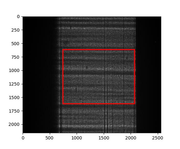
Next let’s use the self-reference XSS technique. Similar to the above examples, we define the Imagestack class imstack, the Tracking class track_XSS and their related parameters in order. Then we call the XSS_self() function.

imstack = Imagestack(sam_folderX, ROI)

track_XSS = Tracking(imstack)
track_XSS.dimension = '1D'
track_XSS.scandim = 'x'
track_XSS.dist = 833.   # [mm]
track_XSS.scanstep = 1.0  # [um]
track_XSS.pixsize = 1.07  # [um]

edge_x = 10
edge_y = 10
edge_z = 10
nstep = 2

track_XSS.XSS_self(edge_x, edge_y, edge_z, nstep, display=False, normalize=True)

Unlike the example of plane mirror measurement with reference beam, in which the XSS technique with reference beam is used, we use the self-reference XSS technique in this example. Thus, the local wavefront curvature other than local wavefront slope is obtained directly from the data processing procedure. Since the speckle generator was scanned in the horizontal direction, the obtained wavefront local curvature is stored in the curv_X attribute of track_XSS class.

We know that the wavefront local curvatur can also be obrained using the self-reference XST technique. Doing the same as in the above, we create a new Tracking class track_XST.

imstack_1 = Imagestack(data_folder, ROI)
imstack_1.fnum = 1
imstack_1.fstart = 0

imstack_2 = Imagestack(data_folder, ROI)
imstack_2.fnum = 1
imstack_2.fstart = 5

track_XST = Tracking(imstack_1, imstack_2)
track_XST.dimension = '1D'
track_XST.scandim = 'x'
track_XST.dist = 833.   # [mm]
track_XST.scanstep = 5.0  # [um]
track_XST.pixsize = 1.07  # [um]

Two images taken at two different diffuser positions are only needed for the self-reference XST technique, we can choose any two images form the scanned dataset. We choose the first (No. 0) image and the sixth (No. 5) image. Thus, the scanstep is 5 \(\mu m\).

edge_x = [20, 20]
edge_y = 10
pad_x = [20, 20]
hw_xy = 15
pad_y = 10

track_XST.XST_self(edge_x, edge_y, pad_x, pad_y, hw_xy, display=False, normalize=True)

To use the XST_self() function to process the data, we need to set some additional parameters properly. Please refer to the user guide for the meaning of these parameters. The obtained wavefront local curvature is also stored in the curvX or curvY attribute. In this case, it is in curvX.

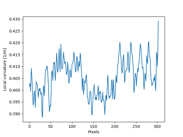
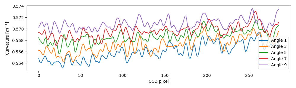
We plot the wavefront curvature obtained from the two technqiues together, note that the way to calculate the wavefront curvature from the two techniques are different, please refer to Local curvature reconstruction.

Wavefront curvature obtained from XSS and XST techniques.

The results from the two techniques match with each other. Further, we can also plot the tracking coefficient. The tracking coefficient is stored in resX and/or resY attribute of Tracking class.

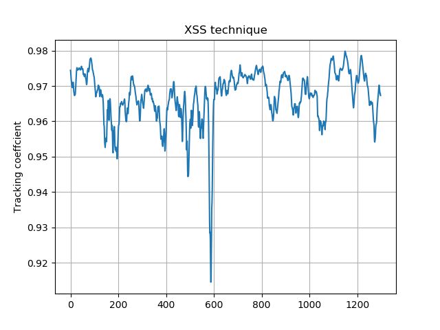
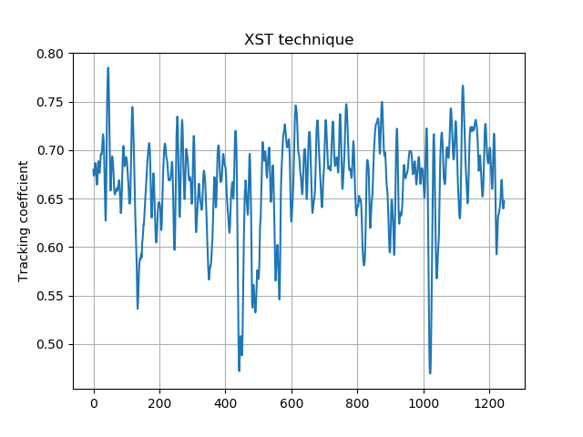
From the tracking coefficients we can find that the XSS technique in general have higher tracking coefficient than the conventional XST technique.

We can also compare the 2D data prcossing method of these two techniques.

track_XSS.dimension = '2D' #'1D'

edge_x = 10
edge_y = 10
edge_z = 10
nstep = 2
pad_xy = 10
hw_xy = 20
cpu_no = 16
#track_XSS.XSS_self(edge_x, edge_y, edge_z, nstep, hw_xy, pad_xy, display=True, normalize=True)
track_XSS.XSS_self_multi(edge_x, edge_y, edge_z, nstep, hw_xy, pad_xy, cpu_no, normalize=True)

Warning

Please check the available CPUs before calling XSS_self_multi() method.

For 2D case of self-reference XSS technique, the original parameters for 1D technique remain the same. Several new parameters need to be added for the XSS_self() or XSS_self_multi() function. Please refer to the user guide for the setting of these parameters. We have the following result of 2D local wavefront curvature map.

Likewise, we can do the 2D data processing for self-reference XST technique. Also, the parameters for 2D processing should be changed in order to have successful tracking result.

track_XST.dimension = '2D' #'1D'

edge_x = [20, 20]
edge_y = [20, 25]
pad_x = [20, 20]
hw_xy = 30
pad_y = [20, 25]
window = 60
cpu_no = 16

#track_XST.XST_self(edge_x, edge_y, pad_x, pad_y, hw_xy, window, display=True, normalize=True)
track_XST.XST_self_multi(edge_x, edge_y, pad_x, pad_y, hw_xy, window, cpu_no, normalize=True)

Warning

Please check the available CPUs before calling XST_self_multi() method.

Note that sometimes the following warning information will pop out,

Potential tracking failure, no subpixel registration:

This is because some subregion changed too much that the tracking fails. Ignore those warnings, we still have the following 2D wavefront map.

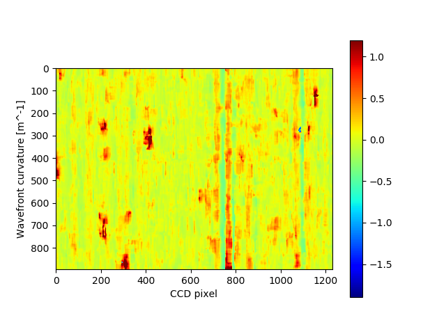
The wavefront curvature map from the self-reference XST technique has lower spatial resolution and accuracy compared to the self-reference XSS technique.

[HuXSTOEPaperFast] (1,2,3)

Hu, L., Wang, H., Fox, O., & Sawhney, K. (2022). Fast wavefront sensing for X-ray optics with an alternating speckle tracking technique. Opt. Exp., 30(18), 33259-33273. https://doi.org/10.1364/OE.460163

KB mirror alignment using self-reference XST technique

Note

Please find the example code from /spexwavepy/examples/KBalignment.py

In this example we will show how to align KB mirror’s pitch angle (\(\theta\)) using the self-reference XST technique. This example is similar to Fig.5 in [HuXSTOEPaperFast].

The basic idea is also described in the above paper. At the nominal angle \(\theta\), the local curvature is constant along the mirror length. However, if it deviates to the nominal value, the local curvature will change along the mirror length. The change of the local curvature can be assumed linealy to the mirror length coordinate.

We first obtain the wavefront curvature for both HKB and VKB using the self-reference XST technique. Note that for this technique, only one image is needed for each image stack, thus, the parameter fnum is 1. In each folder, the two images are at two different diffuser positions. The movement of the diffuser is 4 \(\mu m\). The codes in this example for calling the XST_self() function is similar to the above example.

###### HKB self-reference XST
ROI_HKB = [45, 545, 60, 330]

delayHKB_stack = np.zeros((13, 466))
curvYHKB_stack = np.zeros((13, 466))

for jc in range(1, 14, 1):
    imstack_tmp_1 = Imagestack(folder_prefix_HKB+'theta' + str(jc) + '/', ROI_HKB)
    imstack_tmp_1.fstart = 0
    imstack_tmp_1.fnum = 1

    imstack_tmp_2 = Imagestack(folder_prefix_HKB+'theta' + str(jc) + '/', ROI_HKB)
    imstack_tmp_2.fstart = 1
    imstack_tmp_2.fnum = 1

    track_tmp = Tracking(imstack_tmp_1, imstack_tmp_2)
    track_tmp.dimension = '1D'
    track_tmp.scandim = 'y'
    track_tmp.dist = 1650.0   # [mm]
    track_tmp.scanstep = 4.0   # [um]
    track_tmp.pixsize = 6.45   # [um]

    edge_x = 10
    edge_y = [5, 20]
    pad_x = 10
    pad_y = [5, 20]
    hw_xy = 10

    track_tmp.XST_self(edge_x, edge_y, pad_x, pad_y, hw_xy, display=False, normalize=True)

    delayHKB_stack[jc-1] = track_tmp.delayY
    curvYHKB_stack[jc-1] = track_tmp.curvY

##### VKB self-reference XST
ROI_HKB = [50, 540, 30, 350]

delayVKB_stack = np.zeros((13, 286))
curvYVKB_stack = np.zeros((13, 286))

for jc in range(1, 11, 1):
    imstack_tmp_1 = Imagestack(folder_prefix_HKB+'theta' + str(jc) + '/', ROI_HKB)
    imstack_tmp_1.fstart = 0
    imstack_tmp_1.num = 1

    imstack_tmp_2 = Imagestack(folder_prefix_HKB+'theta' + str(jc) + '/', ROI_HKB)
    imstack_tmp_2.fstart = 1
    imstack_tmp_2.num = 1

    track_tmp = Tracking(imstack_tmp_1, imstack_tmp_2)
    track_tmp.dimension = '1D'
    track_tmp.scandim = 'x'
    track_tmp.dist = 1650.0   # [mm]
    track_tmp.scanstep = 4.0   # [um]
    track_tmp.pixsize = 6.45   # [um]

    edge_x = [20, 5]
    edge_y = 10
    pad_x = [20, 5]
    pad_y = 10
    hw_xy = 10

    track_tmp.XST_self(edge_x, edge_y, pad_x, pad_y, hw_xy, display=False, normalize=True)

    delayVKB_stack[jc-1] = track_tmp.delayX
    curvYVKB_stack[jc-1] = track_tmp.curvX

We then plot the obtained local curvature, which is stored in the curvX and curvY in the Tracking class, for both HKB and VKB.

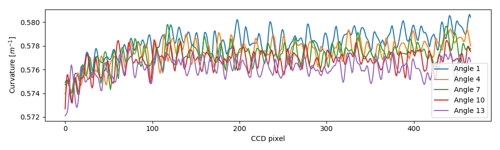
Local wavefront curvature of HKB mirror.

We can find that the data close to one end is abnormal due to the visible stains observed on the mirror surface, we cut that part.

Local wavefront curvature of HKB mirror after cropping the abnormal data.

We do the same for the VKB mirror.

Local wavefront curvature of VKB mirror.

We then do the linear fitting for the measured local wavefront curvature data. From the following figure we can see the linear relation predicted by the theory clearly. The nominal angle \(\theta\) is at the position where the fitted slope is close to 0.

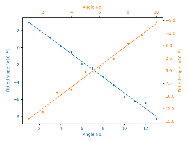
The fitted slope for the above measured curves.

Please refer to the paper [HuXSTOEPaperFast] for more details.

Hartmann-like data processing scheme

Note

Please find the example code from /spexwavepy/examples/Hartmann.py

We have also implemented a speckle-based data processing methods that resemble the conventional Hartmann-like data processing method. We will demonstrate it in this example.

ROI_sam = [540, 1570, 750, 1800]
ROI_ref = ROI_sam

Imstack_sam = Imagestack(, ROI_sam)
Imstack_ref = Imagestack(ref_folder, ROI_ref)
Imstack_sam.read_data()
Imstack_ref.read_data()

For this data processing mode, one reference and one sample image stack are needed. There will be only one image in each image stack.

print(Imstack_sam.data.shape)
print(Imstack_ref.data.shape)

(1, 1030, 1050)
(1, 1030, 1050)

For Hartmann-like data processing mode, we need to define the subregions used for pattern shift tracking. The subregion is a rectangular box. We need to define the centre and the size of each box.

x_cens = np.arange(50, 1050, 50)
y_cens = np.arange(60, 1000, 50)
size = 15

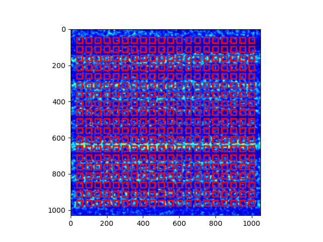
According to the implementation of the Hartmann-like method, the real size for the subregion is \(2 \times size\) for both width and height. We use Hartmann_mesh_show() function to show the subregions defined for the Hartmann-like data processing method. Note the coordinates of the boxes need to be expanded to 2D mesh grid when as the input of the Hartmann_mesh_show() function.

from spexwavepy.corefun import Hartmann_mesh_show

X_cens, Y_cens = np.meshgrid(x_cens, y_cens)
Hartmann_mesh_show(Imstack_ref.data[0], X_cens, Y_cens, size)
plt.show()

The chosen rectangular boxes are shown in red in the following image.

Like other data processing methods, we need to define the Tracking class. Then we invoke the Hartmann_XST() function to obtain the speckle pattern shifts.

Track_Hartmann = Tracking(Imstack_sam, Imstack_ref)
pad = 20
Track_Hartmann.Hartmann_XST(X_cens, Y_cens, pad, size)

The calculated speckle patterns shifts are stored in Tracking.delayX and Tracking.delayY.

plt.figure()
plt.imshow(Track_Hartmann.delayX, cmap='jet')
plt.figure()
plt.imshow(Track_Hartmann.delayY, cmap='jet')

plt.show()

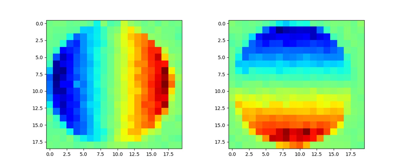
The above results resemble those in the Tutorial. However, the above results have worse spatial resolution.

Unlike the other data processing methods, for Hartmann-like method, we only keep speckle tracking shifts, the physical quantities such as wavefront slope and curvature are left to user to recover. For more detailed description of this method, please refer to the user guide.